Solving second order ODEs
1. AIM: Solving second order ODEs of Simple Pendulum in MATLAB.
2. GOVERNING EQUATIONS:
- ODE of motion of a simple pendulum with damping, `frac{d^2theta}{dt^2}+frac{b}{m}frac{d theta}{d t}+frac{g}{L}sin theta = 0` ...... (A)
- converting eq.(A) into first order differential equation. `frac {d theta_1}{dt}=theta_2`.....(B) & `frac{d theta_2}{dt}=-frac{b}{m}theta_2-frac{g}{L}sin theta_1`....(C)
where, `g` = gravity in `frac{m}{s^2}`
`L` = length of pendulum in `m`.
`m` = mass of the ball in `kg`.
`b` = damping coefficient.
3. OBJECTIVES OF THE PROJECT:
- write a program that will simulate the pendulum motion using this equation,`frac{d^2theta}{dt^2}+frac{b}{m}frac{d theta}{d t}+frac{g}{L}sin theta = 0`
- creating plot/animation of pendulum based on results data.
4. BODY OF THE CONTENT:
INTRODCTION :
A Differential equations are mathematical tools to model engineering systems.An ODE model is a set of differential equations involving functions of only one independent variable and one or more of their derivatives with respect to that variable.
Newton's second law is used in determining the net force on the pendulum by setting the gravitational force equal to the force of the string that pulls back up on the pendulum.
Here is the figure that shows an idealized pendulum, with a "massless" string or rod of length L and a bob of mass m. The open circle shows the rest position of the bob. When the bob is moved from its rest position and let go, it swings back and forth. The time it takes the pendulum to swing from its farthest right position to its farthest left position and back to its next farthest right position is the period of the pendulum.

The primary forces acting on the bob are the gravitational force that makes it move in the first place and the force exerted by the string to keep it moving along a circular path. In addition, there may be a damping force from friction at the pivot or air resistance or both.
Let s(t) be the distance along the arc from the lowest point to the position of the bob at time t, with displacement to the right considered positive. Let theta(t) be the corresponding angle with respect to the vertical. The figure shows tangential and radial components of gravitational force on the pendulum bob. The radial component is exactly balanced by the force exerted by the string, so the only relevant force producing the motion is the tangential component of the gravitational force. For the current moment, we ignore the damping force.
The gravitational force is directed downward and has magnitude mg. Thus, the force acting in the tangential direction is -mg sin(theta).(The negative sign is because this force is in the negative direction when theta is positive and vice versa). Since this force is mass x acceleration, it follows that
`frac{d^2s}{dt^2} = - g sin theta`
Now s and theta are related as arc length and central angle in a circle of radius L: s = L theta. Thus, the second derivative of s is L times the second derivative of theta. That brings us to our undamped model differential equation with a single dependent variable, the angular displacement theta.
`frac{d^2 theta}{dt^2} = - frac{g}{L}sin theta`
Next, we add damping to the model. We make the simplest possible assumption about the damping force, that it is proportional to velocity. Since arc length and central angle are themselves proportional (with proportionality constant L), it makes no difference whether we use linear or angular velocity. Having selected theta as our dependent variable, we will represent the damping as proportional to angular velocity, say, -b (d theta / dt). The negative sign is because the damping force has to be opposite the direction of motion.
`frac{d^2 theta}{dt^2}= - frac{b}{m} frac{d theta}{dt}-frac{g}{L}sin theta`
`therefore`
`frac{d^2theta}{dt^2}+frac{b}{m}frac{d theta}{dt}+frac{g}{L}sin theta = 0` ...... (A)
CONVERTING INTO FIRST ORDER EQUATION :
taken, `theta` = `theta_1` .....(1)
`therefore` `frac{d theta}{dt} = frac{d theta_1}{dt} = theta_2` ......(B)
% simulate the pendulum motion using 2nd ODE.
close all
clear all
clc

% input data
b = 0.05;           % damping coefficient
g = 9.81;           % gravity in m/s2
L = 1 ;             % length of the pendulum in m
m = 1;              % mass of the bob in kg

% initial position of pendulum
theta_0 = [0;3];    % [ respectively, angular displacement in radian ; velocity in rad/sec]

% simulating time range
t_span = [0 20];    % [ respectively starting & end time ]

% solving ODE using ode45 func_handle
% ''ode45(@(t,theta)'' is matlab function handler.
% ''ode_func(t, theta, b,g,L,m)'' ,function code
[t, y] = ode45(@(t,theta) ode_func(t, theta, b,g,L,m),t_span,theta_0);


% plotting curve for displacement,velocity with respect to time
figure(1)
plot(t,y(:,1),'color','red') % giving displacement
hold on
plot(t,y(:,2),'color','black') % giving velocity
legend('displacement','velocity')
title('displacement,velocity vs time')
xlabel('time')
ylabel('displacement & velocity')
grid on
hold off


% Animating the transient motion of the simple pendulum

ct = 1;
for i = 1 : length(y(:,1))
    figure(2)
    x0 = 0;
    y0 = 0;
    x1 =  L*sin(y(i,1))
    y1 =  -L*cos(y(i,1))
    plot([x0 x1],[y0 y1],'color','r')
    hold on
    plot(x1, y1,'o','MarkerSize',20,'color','b')
    axis([-2 2 -2 2])
    pause(0.0001)
    title("animating pendulum")
    grid on
    hold off

% started capturing a plot frame
M(ct) = getframe(gcf);
ct = ct +1
end
%
movie(M);
videofile = VideoWriter('2nd_order_ode_pendulum');
open(videofile)
writeVideo(videofile,M)
close(videofile)
ode_func Function code :
% creating as per equation (D)
function [dtheta_dt] = ode_func (t,theta,b,g,l,m)
theta1 = theta(1)
theta2 = theta(2)
dtheta1_dt = theta2; % eq....(B)
dtheta2_dt = -(b/m)*theta2 - (g/l)*sin(theta1); %eq....(C)
dtheta_dt = [dtheta1_dt; dtheta2_dt]; % eq. (D)
end6. OUTPUT
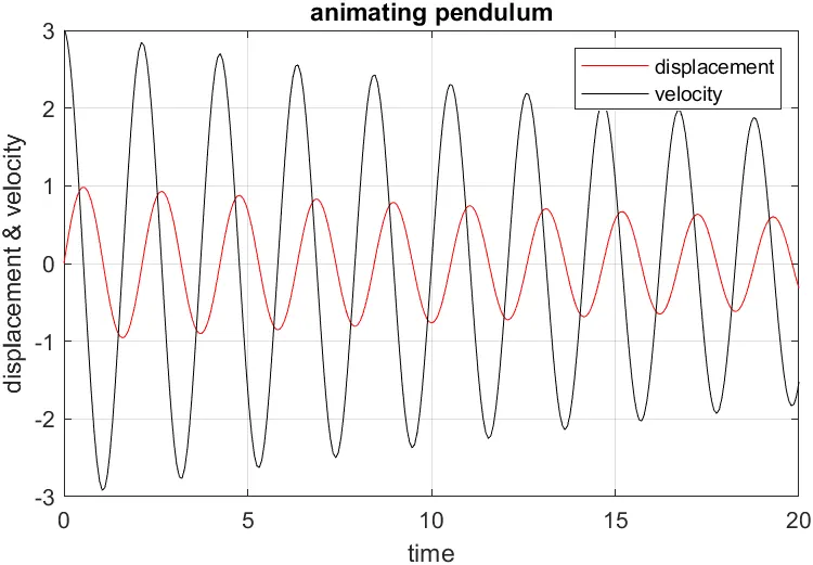
displacement-velocity v/s time graph
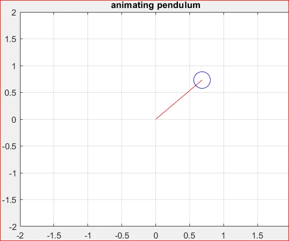
we can see animation of pendulum here.
7. CONCLUSION :
- As, we know, The damper is limiting the amount of vibration/velocity of a system, so, w.r.t by incresing the value of `b`, we can see how quickly the sysyem is damped.
- by this exercise I can solve any ODEs in Matlab.
ERROR WHILE PROGRAMING :
- getting a wrong animation of the plot,
- later,I find out that I used 'sind,cosd' instend of 'sin,cos', beacuse results output in radian.
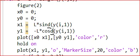
- later,I find out that I used 'sind,cosd' instend of 'sin,cos', beacuse results output in radian.
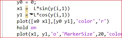
- getting pendulum motion in wrong direction,
- to solve this I putted '-' sign in "y1" equation.