Week 4.1 - Genetic Algorithm
Aim: To optimize the stalagmite function and find the global maxima of the function
Principle :
Stalagmite: A stalagmite is a type of rock formation that rises from the floor of a cave due to the accumulation of material deposited on the floor from ceiling drippings. Stalagmites are typically composed of calcium carbonate but may consist of lava, mud, peat, pitch, sand, sinter, and amber (crystallized urine of packrats).
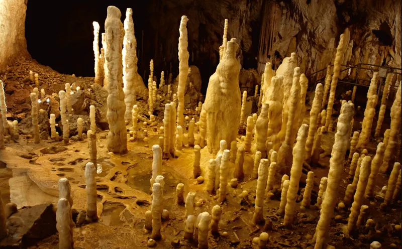
stalagmite formation
A stalagmite in a Matlab is a mathematical function used to generate local maxima and minima. To find a global maximum we need an optimization tool
Introduction to Optimization
Optimization is the process of making something better. In any process, we have a set of inputs and a set of outputs as shown in the following figure.
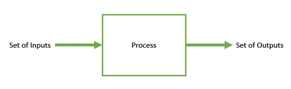
Optimization refers to finding the values of inputs in such a way that we get the “best” output values. The definition of “best” varies from problem to problem, but in mathematical terms, it refers to maximizing or minimizing one or more objective functions, by varying the input parameters.
The set of all possible solutions or values which the inputs can take makes up the search space. In this search space, lies a point or a set of points that gives the optimal solution. Optimization aims to find that point or set of points in the search space.
Genetic Algorithms(GAs) are adaptive heuristic search algorithms that belong to the larger part of evolutionary algorithms. Genetic algorithms are based on the ideas of natural selection and genetics. These are intelligent exploitation of random search provided with historical data to direct the search into the region of better performance in solution space. They are commonly used to generate high-quality solutions for optimization problems and search problems.
Genetic algorithms simulate the process of natural selection which means those species that can adapt to changes in their environment can survive and reproduce and go to the next generation. In simple words, they simulate “survival of the fittest” among individuals of consecutive generations for solving a problem. Each generation consists of a population of individuals and each individual represents a point in search space and a possible solution. Each individual is represented as a string of character/integer/float/bits. This string is analogous to the Chromosome.
The basic structure of a GA is as follows −
We start with an initial population (which may be generated at random or seeded by other heuristics), and select parents from this population for mating. Apply crossover and mutation operators on the parents to generate new off-springs. And finally, these off-springs replace the existing individuals in the population, and the process repeats. In this way, genetic algorithms try to mimic human evolution to some extent.
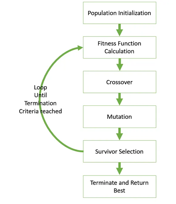
Population Models
There are two population models widely in use −
1 Steady-state
In steady-state GA, we generate one or two off-springs in each iteration and they replace one or two individuals from the population. A steady-state GA is also known as Incremental GA.
2 Generational
In a generational model, we generate ‘n’ off-springs, where n is the population size, and the entire population is replaced by the new one at the end of the iteration.
Operators of Genetic Algorithms
Once the initial generation is created, the algorithm evolves the generation using the following operators
1) Selection Operator: The idea is to give preference to the individuals with good fitness scores and allow them to pass their genes to successive generations.
2) Crossover Operator: This represents mating between individuals. Two individuals are selected using the selection operator and crossover sites are chosen randomly. Then the genes at these crossover sites are exchanged thus creating a completely new individual (offspring)
3) Mutation Operator: The key idea is to insert random genes in offspring to maintain the diversity in the population to avoid premature convergence
A fitness score is the number of characters that differ from characters in the target string at a particular index. So individual having lower fitness value is given more preference.
Matlab Program
Program 1
% Stalagmite function

function[f] = stalagmite(input_vector);

x = input_vector(1);
y = input_vector(2);


 f1x = ((sin(5.1*pi*x+0.5))^6);
  f1y = ((sin(5.1*pi*y+0.5))^6);

  term1 = (((x-0.0667)^2)/0.64);
  term2 = (((y-0.0667)^2)/0.64);
  f2x = exp((-4*log(2))*term1);
    f2y = exp((-4*log(2))*term2);

    f = -(f1x*f1y*f2x*f2y)
end
Program 2:stastical behavior
% Statistical behavior of GA
clear all
close all
clc


x = linspace(0,0.6,150);
y = linspace(0,0.6,150);

[xx,yy] = meshgrid(x,y);

for i = 1:length(xx);
    for j = 1:length(yy);
        input_vector(1) = xx(i,j);
        input_vector(2) = yy(i,j);
         f(i,j)= stalagmite(input_vector);
    end
end

%num of iterations
num_cases =50;

% to find the time required for execution tic toc command is used
tic

for i = 1:num_cases
    [inputs,fopt(i)]= ga(@stalagmite,2);
    xopt(i) = inputs(1);
    yopt(i) = inputs(2);
end
 study_timer = toc

%plotting the stalagamite function of 50 iterations
figure(1)
subplot(2,1,1)
hold on
surfc(xx,yy,f)
shading interp
plot3(xopt,yopt,fopt,'marker','o','markersize',5,'markerfacecolor','r')
title('unboundedinputs')
subplot(2,1,2)
plot(fopt)
xlabel('iterations')
ylabel('functionminimum')
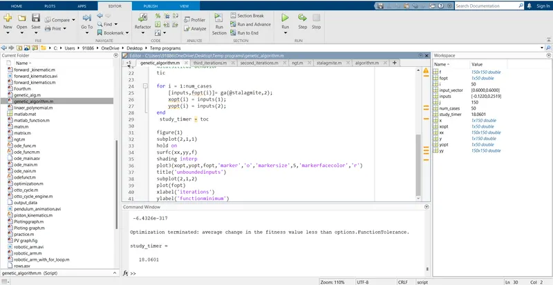
OutPut of the Program 2
Graph
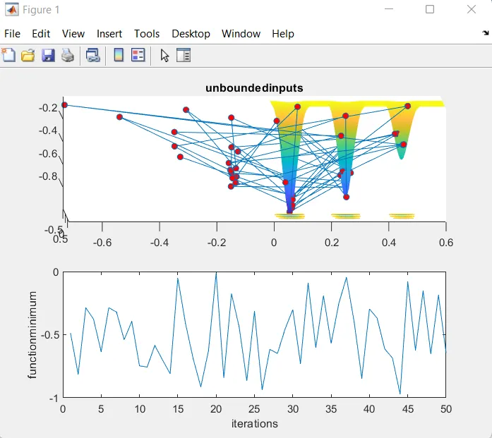
Output screen
Program3 : statistical behavior with upper and lower bounds
clear all
close all
clc


x = linspace(0,0.6,150);
y = linspace(0,0.6,150);

[xx,yy] = meshgrid(x,y);


for i = 1:length(xx);
    for j = 1:length(yy);
        input_vector(1) = xx(i,j);
        input_vector(2) = yy(i,j);
         f(i,j)= stalagmite(input_vector);
    end
end

num_cases =100;

% upper bonds and lower bonds

tic
for i = 1:num_cases
    [inputs,fopt(i)]= ga(@stalagmite,2,[],[],[],[],[0;0],[1;1]) ;
    xopt(i) = inputs(1);
    yopt(i) = inputs(2);
end
Study_timer = toc

figure(1)
subplot(2,1,1)
hold on
surfc(xx,yy,f)
shading interp
plot3(xopt,yopt,fopt,'marker','o','markersize',5,'markerfacecolor','r')
title('unboundedinputs')
subplot(2,1,2)
plot(fopt)
xlabel('iterations')
ylabel('functionminimum')
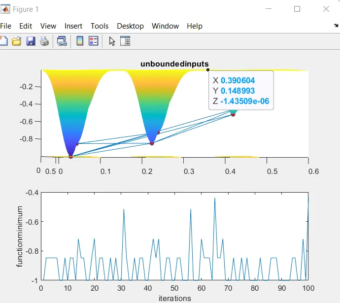
OutPut of the Program 3
Graph
Output screen
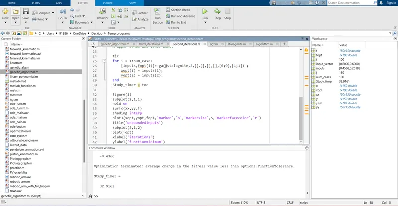
Program 4: increasing the no of populations and iterations
clear all
close all
clc


x = linspace(0,0.6,150);
y = linspace(0,0.6,150);

[xx,yy] = meshgrid(x,y);


for i = 1:length(xx);
    for j = 1:length(yy);
        input_vector(1) = xx(i,j);
        input_vector(2) = yy(i,j);
         f(i,j)= stalagmite(input_vector);
    end
end

num_cases = 150;
options = optimoptions('ga')
options = optimoptions(options,'PopulationSize',300)

tic
for i = 1:num_cases
    [inputs,fopt(i)]= ga(@stalagmite,2,[],[],[],[],[0;0],[1;1],[],[],options)
    xopt(i) = inputs(1);
    yopt(i) = inputs(2);
    opt_f = -fopt
end
Study_timer = toc

figure(1)
subplot(2,1,1)
hold on
surfc(xx,yy,f)
shading interp
plot3(xopt,yopt,fopt,'marker','o','markersize',5,'markerfacecolor','r')
title('unboundedinputs')
subplot(2,1,2)
plot(opt_f)
xlabel('iterations')
ylabel('functionminimum')
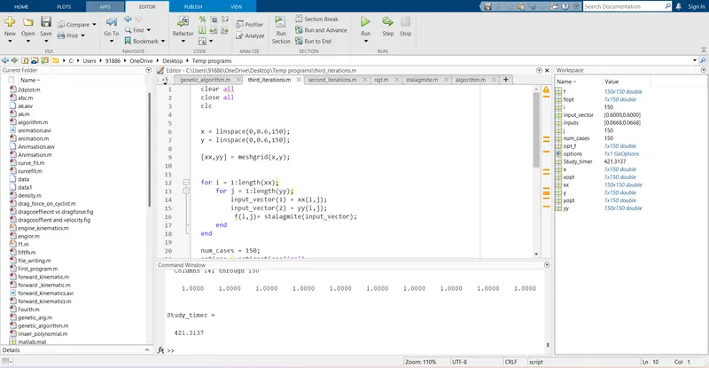
Output of program4
Graph
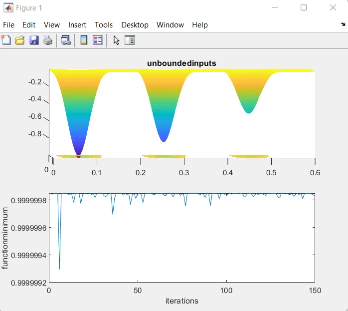
Output Screen
Explanation of the codes
clear all function erases all the variables stored
close all function closes all the graph
clc clears the command wind
The stalagmite function is the subprogram where the stalagmite functions are executed
Num_cases is the no of iterations ga has to be executed
Tic and toc command is used to record the time required to execute the program
ga command is used for the genetic algorithm
subplot command is so that both graphs appear in the same window
surfc command gives the contour graph
shading interp prevents the shading of the graph
xlabel command determines the name of the x-axis
ylabel command determines the name of the y-axis
when the Program 2 is executed the minimum value of the ga function is all over the place and the value is not repeated hence we have to fix the upper and lower bounds
Youtube link : https://youtu.be/kHyNqSnzP8Y