Project 2 - Rankine cycle Simulator

Aim: To create a Rankine cycle stimulator using Matlab

Principle: The Rankine cycle is an idealized thermodynamic cycle describing the process by which certain heat engines, such as steam turbines or reciprocating steam engines, allow mechanical work to be extracted from a fluid as it moves between a heat source and heat sink. The Rankine cycle is named after William John Macquorn Rankine, a Scottish polymath professor at Glasgow University.

The steps in the Rankine Cycle as shown in Figure 1 and the corresponding steps in the pressure-volume diagram (figure 2) are outlined below:

• Pump: Compression of the fluid to high pressure using a pump (this takes work) (Figure 2: Steps 3 to 4)
• Boiler: The compressed fluid is heated to the final temperature (which is at boiling point), therefore, a phase change occurs—from liquid to vapor. (Figure 2: Steps 4 to 1)
• Turbine: Expansion of the vapor in the turbine. (Figure 2: Steps 1 to 2)
• Condenser: Condensation of the vapor in the condenser (where the waste heat goes to the final heat sink (the atmosphere or a large body of water (ex. lake or river)

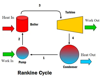
Figure(1): A simple schematic with components for the Rankine Cycle.

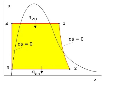
Figure(2): The pressure-volume diagram of the Rankine cycle.

There are four processes in the Rankine cycle.

• Process 1–2: The working fluid is pumped from low to high pressure. As the fluid is a liquid at this stage, the pump requires little input energy. Process 1-2 is isentropic compression.
• Process 2–3: The high-pressure liquid enters a boiler, where it is heated at constant pressure by an external heat source to become a dry saturated vapor. The input energy required can be easily calculated graphically, using an enthalpy–entropy chart (h–s chart, or Mollier diagram), or numerically, using steam tables or software. Process 2-3 is constant pressure heat addition in the boiler.
• Process 3–4: The dry saturated vapor expands through a turbine, generating power. This decreases the temperature and pressure of the vapor, and some condensation may occur. The output in this process can be easily calculated using the chart or tables noted above. Process 3-4 is isentropic expansion.
• Process 4–1: The wet vapor then enters a condenser, where it is condensed at a constant pressure to become a saturated liquid. Process 4-1 is constant pressure heat rejection in the condenser.

In general, the efficiency of a simple Rankine cycle can be written as

Each of the next four equations is derived from the energy and mass balance for a control volume. defines the thermodynamic efficiency of the cycle as the ratio of net power output to heat input. As the work required by the pump is often around 1% of the turbine work output, it can be simplified.

When dealing with the efficiencies of the turbines and pumps, an adjustment to the work terms must be made:

Main Code

clear all 
close all
clc
 
fprintf('1-2:isentropic compression\n')
fprintf('2-3:Constant pressure Heat addition\n')
fprintf('3-4:isentropic expansion\n')
fprintf('4-1:constant Pressure Heat rejection\n')

%input
p1 = input('Enter the turbine inlet pressure')
t1 = input('Enter the turbine inlet temperature')
p2 = input('Enter the turbine oulet pressure')

%state variable at 1
H1 = XSteam('h_pt',p1,t1)
S1 = XSteam('s_pt',p1,t1)
SL1 = XSteam('sL_p',p1)
SV1 = XSteam('sV_p',p1)
T_sat1 = XSteam('Tsat_p',p1)


%state variable at 2
S2 = S1
SL2 = XSteam('sL_p',p2)
SV2 = XSteam('sV_p',p2)
HL2 = XSteam('hL_p',p2)
HV2 = XSteam('hv_p',p2)
DF = ((S2-SL2)/(SV2-SL2))
H2 = HL2+DF*(HV2-HL2)
t2 = XSteam('T_ph',p2,H2)
T_sat = XSteam('Tsat_p',p2)

%state variable at 3
t3 = t2
p3 = p2
S3 = XSteam('sL_T',t3)
H3 = XSteam('hL_T',t3)
V3 = XSteam('vL_p',p2)

%State variable at 4
p4 = p1
S4 = S3
CP4 = XSteam('Cp_ps',p4,S4)
CV4 = XSteam('Cv_ps',p4,S4)
gamma = CP4/CV4
r = (gamma-1)/gamma
t4 = t3*(p4/p3)*r

%Work done by the turbine
WT = H1-H2

%work done by the pump

WP = V3*(p1-p2)*100
H4 = WP+H3

%Net Work

W_NET = WT-WP

%efficiency

n = (W_NET/(H1-H4))*100

%Back work ratio

R = WP/WT

%specific Heat conductivity

SSC = 3600/WT

%Displaying the output
disp('        Results    ');
disp('At state point 1');
fprintf('P1 is : %.2f Bar \n',p1);
fprintf('T1 is : %.2f Deg Celcius \n',t1);
fprintf('H1 is : %.2f KJ/kg \n',H1);
fprintf('S1 is : %.2f KJ/kgk \nn',S1);

disp('At state point 2');
fprintf('P2 is : %.2f Bar \n',p2);
fprintf('T2 is : %.2f Deg Celcius \n',t2);
fprintf('H2 is : %.2f KJ/kg \n',H2);
fprintf('S2 is : %.2f KJ/kgk \nn',S2);

disp('At state point 3');
fprintf('P3 is : %.2f Bar \n',p3);
fprintf('T3 is : %.2f Deg Celcius \n',t3);
fprintf('H3 is : %.2f KJ/kg \n',H3);
fprintf('S3 is : %.2f KJ/kgk \nn',S3);

disp('At state point 4');
fprintf('P4 is : %.2f Bar \n',p4);
fprintf('T4 is : %.2f Deg Celcius \n',t4);
fprintf('H3 is : %.2f KJ/kg \n',H4);
fprintf('S4 is : %.2f KJ/kgk \nn',S4);

fprintf('work done by the turbine is: %.2f KJ/kg \n',WT);

fprintf('work done by the pump is : %.2f kj/kg \n',WP);

fprintf('net work is : %.2f KJ/kg \n',W_NET);
 
fprintf('thermal efficiency is : %.2f % \n',n);

fprintf('Back Work ratio is : %.2f \n',R);

fprintf('Specific steam conductivity is :%.2f kg/KWH \n',SSC);

%PLotting the graphs

t = linspace(0,400,200);
figure(1)
hold on

for i = 1:length(t)
    plot(XSteam('sL_T',t(i)),t(i),'r.')
    plot(XSteam('sV_T',t(i)),t(i),'r.')
end

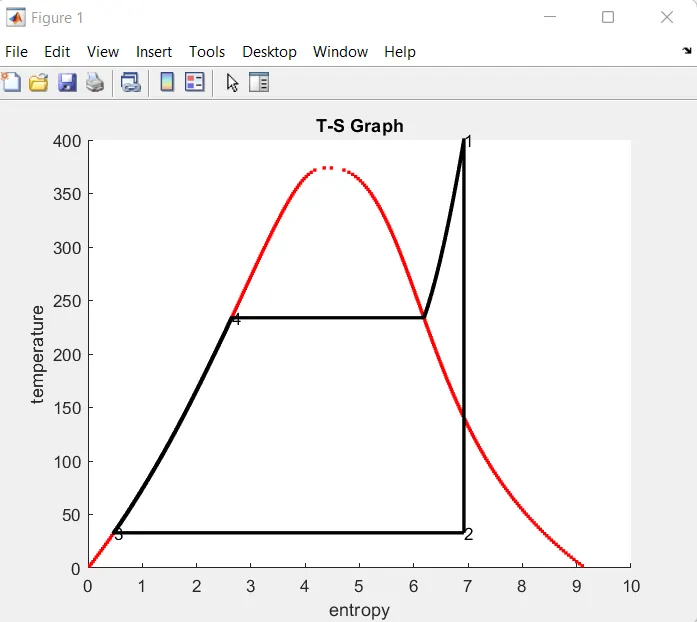
plot([S1 S2],[t1 t2],'linewidth',2,'color','k')
text(S1,t1,'1','FontSize',10)
if DF>1
t3 = T_sat;
plot([S2 SV2 S3 S4],[t2 T_sat t3 t4],'linewidth',2,'color','k')
t2 = T_sat;
text(S2,t2,'2','FontSize',10)
text(S3,t3,'3','FontSize',10)
else
plot([S2 S3],[t2 t3 ],'linewidth',2,'color','k')
text(S2,t2,'2','FontSize',10)
text(S3,t3,'3','FontSize',10)
end

m = linspace(t1,t2,500)
for i= 1:length(m)
plot(XSteam('s_pT',p1,m(i)),m(i),'.','linewidth',2,'color','k')
end

plot([SL1 SV1],[T_sat1 T_sat1],'linewidth',2,'color','k')
text(SL1,T_sat1,'4','fontsize',10)
xlabel('entropy')
ylabel('temperature')
title('T-S Graph')

figure(2)
hold on
for j = 1:length(t)
    plot(XSteam('sL_T',t(j)),XSteam('hL_T',t(j)),'b.')
    plot(XSteam('sV_T',t(j)),XSteam('hV_T',t(j)),'b.')
end
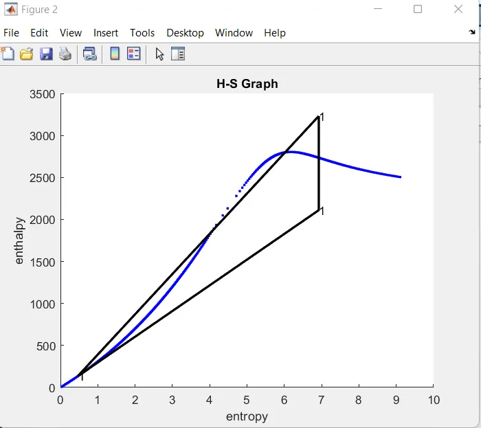
plot([S1 S2 S3 S4 S1],[H1 H2 H3 H4 H1],'linewidth',2,'color','k')
text(S1,H1,'1','FontSize',10)
text(S2,H2,'1','FontSize',10)
text(S3,H3,'1','FontSize',10)
text(S4,H4,'1','FontSize',10)
xlabel('entropy')
ylabel('enthalpy')
title('H-S Graph')
 
 

Explanation of the code:

Clear all command clears variables

Close all closes the graphs

clc clears the command window

fprintf commands prints the input in the command window

input command allows the user to input the value

XSteam is the calling function in which the user can call the required values

Plot commad plots the graph of required values

Font size setermines the size of the text

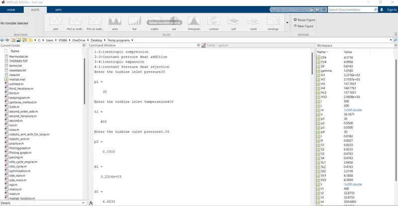
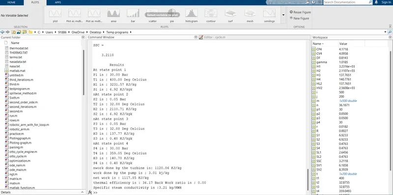
Output Screen:

Graphs: