Report on Use Genetic Algorithm in Matlab to find global maxima

What is a Genetic Algorithm?

Genetic algorithms (GA) are a method of optimization involving iterative search procedures based on an analogy with the process of natural selection (Darwinism) and evolutionary genetics.

Genetic Algorithm Applications

Some examples of GA applications include optimizing decision trees for better performance, automatically solving sudoku puzzles, hyperparameter optimization, etc. In a genetic algorithm, a population of candidate solutions (called individuals, creatures, organisms, or phenotypes) to an optimization problem is evolved toward better solutions.

Genetic Algorithm consists of a class of probabilistic optimization algorithms. GENETIC ALGORITHM MATLAB tool is used in computing to find approximate solutions to optimization and search problems. A set of possible solutions are randomly generated to a problem, each as a fixed-length character string.

A genetic algorithm (GA) is a method for solving both constrained and unconstrained optimization problems based on a natural selection process that mimics biological evolution. The algorithm repeatedly modifies a population of individual solutions. At each step, the genetic algorithm randomly selects individuals from the current population and uses them as parents to produce the children for the next generation. Over successive generations, the population "evolves" toward an optimal solution.

Aim

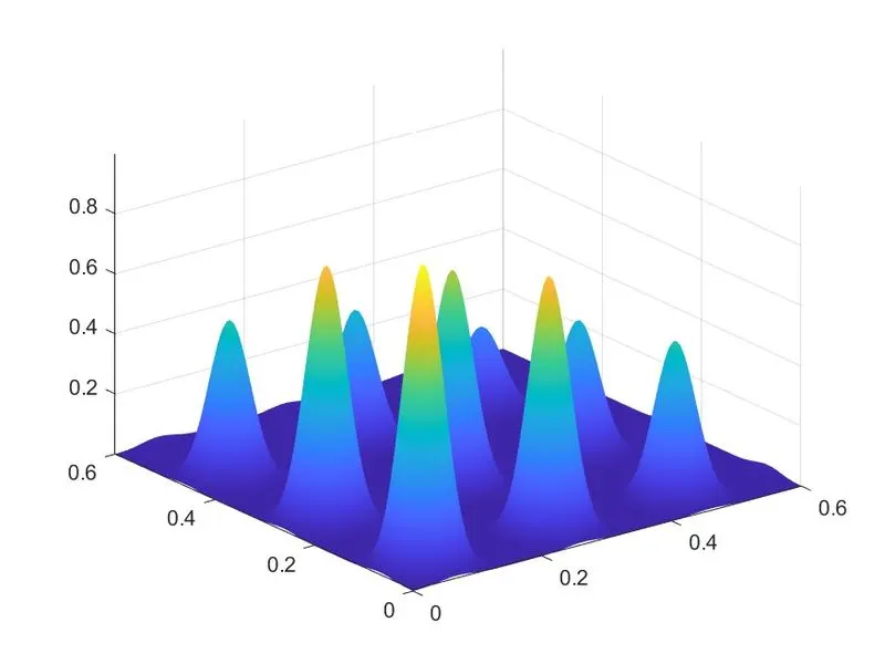
Optimize the stalagmite function and find the global maxima of the function.

Objective

Our objective is to optimize the stalagmite function and find global maxima of the function using different methods and syntax of Gentic Algorithm.

Syntax for ga

x = ga(fun,nvars)

finds a local unconstrained minimum, x, to the objective function, fun. nvars is the dimension (number of design variables) of fun.

x = ga(fun,nvars,A,b)

finds a local minimum x to fun, subject to the linear inequalities A*x ≤ b. ga evaluates the matrix product A*x as if x is transposed (A*x').

x = ga(fun,nvars,A,b,Aeq,beq)

finds a local minimum x to fun, subject to the linear equalities Aeq*x = beq and A*x ≤ b. (Set A=[] and b=[] if no linear inequalities exist.) ga evaluates the matrix product Aeq*x as if x is transposed (Aeq*x').

x = ga(fun,nvars,A,b,Aeq,beq,lb,ub)

defines a set of lower and upper bounds on the design variables, x, so that a solution is found in the range lb ≤ x ≤ ub. (Set Aeq=[] and beq=[] if no linear equalities exist.)

x = ga(fun,nvars,A,b,Aeq,beq,lb,ub,nonlcon)

subjects the minimization to the constraints defined in nonlcon. The function nonlcon accepts x and returns vectors C and Ceq, representing the nonlinear inequalities and equalities respectively. ga minimizes the fun such that C(x) ≤ 0 and Ceq(x) = 0. (Set lb=[] and ub=[] if no bounds exist.)

x = ga(fun,nvars,A,b,Aeq,beq,lb,ub,nonlcon,options)

minimizes with the default optimization parameters replaced by values in options. (Set nonlcon=[] if no nonlinear constraints exist.) Create options using optimoptions.

x = ga(fun,nvars,A,b,Aeq,beq,lb,ub,nonlcon,intcon) or

x = ga(fun,nvars,A,b,Aeq,beq,lb,ub,nonlcon,intcon,options)

requires that the variables listed in intcon take integer values.

x = ga(problem)

finds the minimum for the problem, a structure described in the problem.

[x,fval] = ga(___)

for any previous input arguments, also returns fval, the value of the fitness function at x.

[x,fval,exitflag,output] = ga(___)

also returns an exit flag, an integer identifying the reason the algorithm terminated, and output, a structure that contains output from each generation and other information about the performance of the algorithm.

[x,fval,exitflag,output,population,scores] = ga(___)

also returns a matrix population, whose rows are the final population, and a vector scores, the scores of the final population.

MatLab Program

Program for Basic of ga

clear all 
close all
clc
 
%dedfining our search space 
x = linspace(0,0.6,150);
y = linspace(0,0.6,150);

%creating a 2D mesh
[xx yy] = meshgrid(x,y);
num_cases = 50;

% Evaluating stalagmite function    
for i=1:length(xx)
    for j=1:length(yy)
        input_vector(1)=xx(i,j);
        input_vector(2)=yy(i,j);
        f(i,j)=stalagmite(input_vector);
    end
end

surfc(x,y,-f)       %plotting the surface plot
shading interp      % making smooth surface

[inputs, fval]=ga(@stalagmite, 2)             %finding minimum value of function ga

saveas(gcf,'stalagmite plot.jpg')             %saving plot as image

Explanation:

1. Defining inputs x and y using linspace() command.
2. Creating 2D array using meshgrid() function.
3. Evaluate Stalagmite function for each value of x and y using for loop.
4. Defining input array as row matrix giving input_value variable.
5. Defining stalagmite function.
6. Plot surface of x, y and f.
7. Using [input,fval]=ga(function,variable) we are finding minimum value of ‘ f ’ for inputs of x and y.

Result:

Program for Stalagmite Function

function [f] = stalagmite(input_vector)
x=input_vector(1);
y=input_vector(2);

f1x = [sin(5.1*pi*x+0.5)]^6;
f1y = [sin(5.1*pi*y+0.5)]^6;
f2x = exp(-4*log(2)*((x-0.0667)^2/0.64));
f2y = exp(-4*log(2)*((y-0.0667)^2/0.64));

f = -f1x*f1y*f2x*f2y;
end

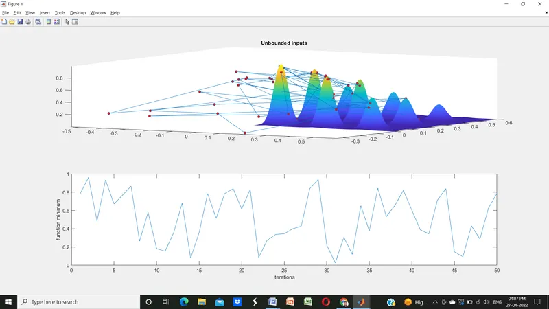
Program For Study 1: Statistical Behavior

clear all 
close all
clc
 
%dedfining our search space 
x = linspace(0,0.6,150);
y = linspace(0,0.6,150);

%creating a 2D mesh
[xx yy] = meshgrid(x,y);
num_cases = 50;

% Evaluating stalagmite function
for i=1:length(xx)
    for j=1:length(yy)
        input_vector(1)=xx(i,j);
        input_vector(2)=yy(i,j);
        f(i,j)=stalagmite(input_vector);
    end
end

surfc(x,y,-f)
shading interp

%Study1-Statistatical Behaviour
tic
for i= 1:num_cases
    [input, fopt(i)] = ga(@stalagmite, 2);
    xopt(i)=input(1);
    yopt(i)=input(2);
end
Study1_time = toc

figure(1)
subplot(2,1,1)
hold on
surfc(x,y,-f)
shading interp
plot3(xopt,yopt,-fopt,'marker','o','MarkerSize',5,'markerfacecolor','r')
title('Unbounded inputs')
subplot(2,1,2)
plot(-fopt)
xlabel('iterations')
ylabel('function minimum')

Explanation:

1. To obtain optimum results we iterating ga for many times using for loop.
2. Using for loop we are doing iteration over 50 times and storing results in fpot for xopt and yopt.
3. Using tic and toc we are calculating running time of code.
4. We used subplot to plot surface and points of fopt, xopt, yopt and fopt against iterations for camparison.

Result:

Program for Study 2: Bounded inputs

clear all 
close all
clc
 
%dedfining our search space 
x = linspace(0,0.6,150);
y = linspace(0,0.6,150);

%creating a 2D mesh
[xx yy] = meshgrid(x,y);
num_cases = 50;

% Evaluating stalagmite function
for i=1:length(xx)
    for j=1:length(yy)
        input_vector(1)=xx(i,j);
        input_vector(2)=yy(i,j);
        f(i,j)=stalagmite(input_vector);
    end
end

surfc(xx,yy,-f)
shading interp
[inputs, fval]=ga(@stalagmite, 2)

tic
for i= 1:num_cases
    [input, fopt(i)] = ga(@stalagmite, 2,[],[],[],[],[0;0],[0.3;0.3]);
    xopt(i)=input(1);
    yopt(i)=input(2);
end
Study1_time = toc

figure(1)
subplot(2,1,1)
hold on
surfc(x,y,-f)
shading interp
plot3(xopt,yopt,-fopt,'marker','o','MarkerSize',5,'markerfacecolor','r')
title('Bounded inputs')
subplot(2,1,2)
plot(-fopt)
xlabel('iterations')
ylabel('function maximum')

Explanation:

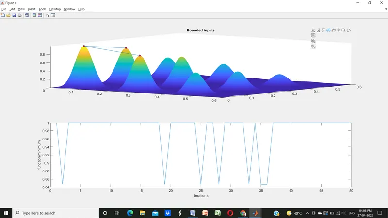
1. All thing are same as study we are just dealing ga syntax.
2. We are using syntax x= ga(fun,nvars,A,b,Aeq,beq,lb,ub) defines a set of lower and upper bounds on the variables, x & y so that a solution is found in the range lb ≤ x,y ≤ ub. (Set Aeq=[] and beq=[] if no linear equalities exist.)
3. As there is no no linear equalities and non-linear equalities exist we leave it blank i.e. A=[], b=[], Aeq=[], beq=[].

Result:

Program for Bounded Inputs with Modified Population Size

clear all 
close all
clc
 
%dedfining our search space 
x = linspace(0,0.6,150);
y = linspace(0,0.6,150);

%creating a 2D mesh
[xx yy] = meshgrid(x,y);
num_cases = 50;

% Evaluating stalagmite function
for i=1:length(xx)
    for j=1:length(yy)
        input_vector(1)=xx(i,j);
        input_vector(2)=yy(i,j);
        f(i,j)=stalagmite(input_vector);
    end
end

surfc(xx,yy,-f)
shading interp
[inputs, fval]=ga(@stalagmite, 2)

%study3- Increasing GA iterations
options = optimoptions('ga');
options = optimoptions(options,'PopulationSize',300);

tic
for i= 1:num_cases
    [input, fopt(i)] = ga(@stalagmite, 2,[],[],[],[],[0;0],[0.3;0.3],[],[],options);
    xopt(i)=input(1);
    yopt(i)=input(2);
end
Study1_time = toc

figure(1)
subplot(2,1,1)
hold on
surfc(x,y,-f)
shading interp
plot3(xopt,yopt,-fopt,'marker','o','MarkerSize',5,'markerfacecolor','r')
title('Bounded inputs with Modified Population size')
subplot(2,1,2)
plot(-fopt)
xlabel('iterations')
ylabel('function maximum')

Explanation:

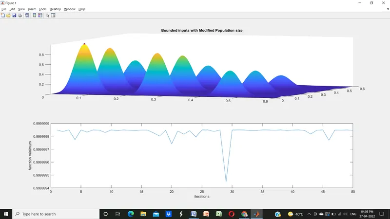
1. Just by changing syntax for ga we can add population size.
2. Using syntax ,x = ga(fun,nvars,A,b,Aeq,beq,lb,ub,nonlcon,intcon,options)minimizes with the default optimization parameters replaced by values in options. ( nonlcon=[] as no nonlinear constraints exist.)
3. Create optionsusing optimoptions.
4. By using – sign to fopt we reversed it in maxima.

Result:

Conclusion:

We can optimize the solution using different methods 1. Using upper and lower bounding of inputs. 2. Controlling the population size of the solution. We need to use proper syntax for the same.

Reference:

1. https://matlab-code.org/genetic-algorithm-matlab
2. https://en.wikipedia.org/wiki/Genetic_algorithm
3. https://in.mathworks.com
4. Youtube Channel: Gate smashers
5. Youtube Channel MATLAB