Report on Solving 2^nd ODEs for Simple Pendulum and obtain plot & Animation of Simple Pendulum using Matlab

       The Differential equations have wide applications in various engineering and science disciplines. In general, modeling the variation of a physical quantity, such as temperature, pressure, displacement, velocity, stress, strain, current, voltage, or concentration of a pollutant, with the change of time or location, or both would result in differential equations. Similarly, studying the variation of some physical quantities on other physical quantities would also lead to differential equations. Many engineering subjects, such as mechanical vibration or structural dynamics, heat transfer, or the theory of electric circuits, are founded on the theory of differential equations. It is practically important for engineers to be able to model physical problems using mathematical equations, and then solve these equations so that the behavior of the systems concerned can be studied. In Engineering, ODE is used to describe the transient behavior of a system. A simple example is a pendulum.

Aim

To solve second order ODEs for a simple pendulum and obtain the plots of results and animation of a simple pendulum.

Governing Equation

 A pendulum is a body suspended from a fixed point so that it can swing back and forth under the influence of gravity. The time interval of a pendulum’s complete back-and-forth movement is constant.

                                            

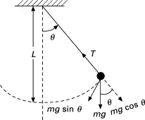
The second-order differential equation ODE for the simple pendulum

Where,

b = damping coefficient

m = mass of the bob kg,

g = acceleration due to gravity m/

l = length of the string m.

please refer the attached report for detailed solved equations.

The simple pendulum problem can be solved by using the second-order ODE functions and by solving these we will get the 𝜃1 and 𝜃2 values of the simple pendulum.

Objective

 Our objective is to write a program that solves the following ODE. This ODE represents the equation of motion of a simple pendulum with damping

MatLab Program

Program for solving ODE function using ode45 solver

close all
clear all 
clc

%Inputs
b=0.05;  %damping Coefficeint      
g=9.81;  %acceleration due to gravity in m/s^2
l=1;     %length of the pendulum in meter
m=1;     %mass of the bob of pendulum in kg

%initial condition
theta_0 = [0;3];     %dedining initial condition of ODE equations that we are solving i.e diplacement is 0 & velocity is 3

%time points
t_span = linspace(0,20,200);       %time array to integrate the 

%solve ODE
[t, results] = ode45(@(t,theta) ode_func(t,theta,b,g,l,m),t_span,theta_0);  %solving ODEs using ode45 solver

%plot
figure(1)
plot(t, results(:,1)) %plotting results of time and displacement
hold on
plot(t,results(:,2))  %plotting results of time and velocity
xlabel('time')        %labeling axes 
ylabel('plot')
grid on
legend('displacement','velocity') 
saveas(gcf,'Results vs time.jpg');

%animation
x0=0;             %coordinates of fixed point
y0=0;
ct=1;              %giving counter to get frame

for i=1:length(t)             %defining number iterations to be done            
    x1=l*sin(results(i,1));   %plotting points at bob
    y1=-l*cos(results(i,1));
    
    figure(2)
    %plotting
   plot([-1 1],[0 0],'LineWidth',4,'color','g');   %plot of supporting rod
   axis([-1.5 1.5 -1.5 0.5]);                      %setting axis limit to show
   line([x0 x1],[y0 y1],'linewidth',1);            %plotting string of lenth l
   hold on
   plot(x1, y1,'O','MarkerSize',10,'MarkerFaceColor','r');   %plotting bob
   plot(x0, y0,'O','MarkerSize',3,'markerfacecolor','r');    %plotting fixed point
   title('Damping of Simple Pendulum');                      %naming the figure
   plot([0 0],[-1 0],'LineStyle','--')
   legend('Supporting rod','String of Pendulum','Bob of pendulum','Fixed point');
   grid on
   hold off 
  
   M(ct)= getframe(gcf);     %storing all the figures at array M
   ct=ct+1;                  %increasing counter
end

movie(M);                   % Stiching all the figures stored in M array to create animation
videofile = VideoWriter('Damping of pendulum','MPEG-4');  %assigning video name and format
open(videofile);    
writeVideo(videofile,M);     %convert images into video 
close(videofile);

Program for function:

function [dtheta_dt] = ode_func(t,theta,b,g,l,m)    %defining function and inputs

theta1 = theta(1);       %assigning value of theta1 
theta2 = theta(2);       %assigning value of theta2
dtheta1_dt = theta2;     %defining first ODE
dtheta2_dt = -(b/m)*theta2 - (g/l)*sin(theta1);   %defining Secound ODE
dtheta_dt = [dtheta1_dt; dtheta2_dt];             %combining ODE to solve in the form of column matrix
end     

Explanation:

1. First we converted 2^nd order ODE into two 1^st order ODEs by putting appropriate values.
2. Inputs like damping coefficient, acceleration due to gravity, length of the pendulum, and mass of bob are given to the program.
3. Then we defined the initial condition from which we are going to integrate a function over a period which is also defined under using the linspace() command.
4. We solve ODEs using ode45() solver, within ode45() solver defined our ODEs are a function of time ‘t’ and ‘theta’ and then called function and defined the period over integration has to be done and initial condition from which integration has to start.
5. Solutions are stored in an array of results for the corresponding time.
6. The plot is made using the plot() command for results of velocity and displacement.
7. Axis were labelled using xlable() & ylable() command.
8. Function program:
9. Using function we defined the ODE function of inputs time, theta, b, g, l, m.
10. Assigning a value of theta1 and theta2 stored in array theta which is a column matrix.
11. Defined ODEs which are converted in 1^st order ODEs.
12. Combined ODEs are defined at the last and then end of the function program.
13. For animation we need to use for loop as we have to obtain different figures for each value of time.
14. Values x0 and y0 are provided which is (0,0)
15. Counter is given to obtain frame.
16. For loop open
17. For each value of ‘i’ it goes from 1 to the length of array ‘t’ we will calculate the value of x1 and y1 as per the formula which is the point at bob suspended to the pendulum.
18. Now using the plot() command we plotted the supporting rod.
19. Then line() command is used to plot the string of the pendulum.
20. Using plot() command ‘markersize’ and ‘matekercolor’ we modified the animation, and coloring of the bob at (x1,y1) at a fixed point of suspension(x0,y0).
21. Also plotted mean line position for better visuals of displacement.
22. Using the get frame() command we stored all current figure frames in array M.
23. Increasing counter by 1 to get the next frame.
24. Movie() command is used to stitch all figure images stored in M to create animation.
25. Using the VideoWriter() command video name and format are given and assigned as a variable called videofile.
26. Then we open the video file, images stitched together are converted using the command writeVideo(), and then close the video file.

Results

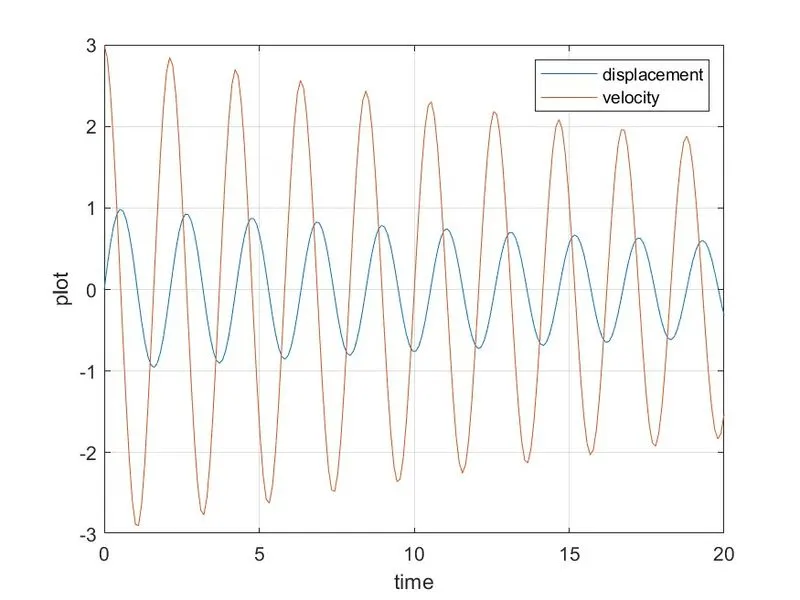
We obtain two results here one is a plot of results i.e. velocity and displacement vs time and the second is an animation of the oscillating pendulum.

For animation link is:

                         

The plot result is:

             

Errors and their solutions

Usually, I did not come across any errors except unusual plots animation which I corrected easily and instantly.

References:

1. Engineering applications of Differential Equations by B. Sumithra.
2. Khan physics academy, Youtube Channel
3. CodingOwl, Youtube Channel

THANK YOU