Week 4.1 - Genetic Algorithm

Aim :- To write a program in MATLAB to optimise the stalagmite function and find the global maxima of the function.

Theory :-

Optimization

Optimization is the process of making something as good or effective as possible. Mathematical optimization is the selection of a best element, with regard to some criterion, from some set of available alternatives. function optimization describes a class of problems for finding the input to a given function that results in the minimum or maximum output from the function.

Genetic algorithms

Genetic algorithms came from the research of John Holland, in the University of Michigan, in 1960. The genetic algorithm is a method for solving both constrained and unconstrained optimization problems that is based on natural selection, the process that drives biological evolution. The genetic algorithm repeatedly modifies a population of individual solutions. At each step, the genetic algorithm selects individuals from the current population to be parents and uses them to produce the children for the next generation. Over successive generations, the population "evolves" toward an optimal solution.

Terminology of Genetic algorithm is as follows

Population: Population is the subset of all possible or probable solutions, which can solve the given problem.

Chromosomes: A chromosome is one of the solutions in the population for the given problem, and the collection of gene generate a chromosome.

Gene: A chromosome is divided into a different gene, or it is an element of the chromosome.

Allele: Allele is the value provided to the gene within a particular chromosome.

Fitness Function: The fitness function is used to determine the individual's fitness level in the population. It means the ability of an individual to compete with other individuals. In every iteration, individuals are evaluated based on their fitness function.

Genetic Operators: In a genetic algorithm, the best individual mate to regenerate offspring better than parents. Here genetic operators play a role in changing the genetic composition of the next generation.

The genetic algorithm works on the evolutionary generational cycle to generate high-quality solutions. These algorithms use different operations that either enhance or replace the population to give an improved fit solution.

It basically involves five phases to solve the complex optimization problems, which are given as below:

• Initialization
• Fitness Assignment
• Selection
• Reproduction
• Termination

Advantages of Genetic algorithm

1. The parallel capabilities of genetic algorithms are best.
2. It helps in optimizing various problems such as discrete functions, multi-objective problems, and continuous functions.
3. It provides a solution for a problem that improves over time.
4. A genetic algorithm does not need derivative information.

Limitations of Genetic algorithm

1. Genetic algorithms are not efficient algorithms for solving simple problems.
2. It does not guarantee the quality of the final solution to a problem.
3. Repetitive calculation of fitness values may generate some computational challenges.

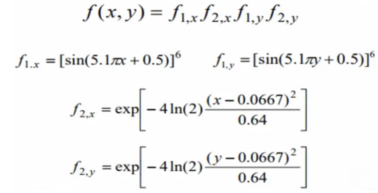
Stalagmite function :-

Program :-

close all
clear all
clc

%Defining our search space
x=linspace(0,0.6,150);
y=linspace(0,0.6,150);
num_cases=30;

%creating a 2 dimensional mesh
[xx yy]=meshgrid(x,y);

%evaluating the stalagmite function
for i=1:length(xx)
    for j=1:length(yy)
        input_vector(1)=xx(i,j);
        input_vector(2)=yy(i,j);
       f(i,j)=stalagmite(input_vector);
    end
end

tic

for i=1:num_cases

[input,fval(i)]=ga(@stalagmite,2);
xopt(i)=input(1);
yopt(i)=input(2);

end
case_time_1=toc

figure(1)
subplot(2,1,1)
surfc(xx,yy,-f)
xlabel('x value')
ylabel('y value')
title('case 1 (Unbounded inputs)')
shading interp
hold on;
plot3(xopt,yopt,-fval,'Marker','o','MarkerSize',5,'markerfacecolor','r')
subplot(2,1,2)
plot(-fval);
xlabel('No of Iterations')
ylabel('max function value')

%case 2
tic
for i=1:num_cases
[input,fval(i)]=ga(@stalagmite,2,[],[],[],[],[0;0],[0.6;0.6]);
xopt(i)=input(1);
yopt(i)=input(2);
end
case_time_2=toc
figure(2)
subplot(2,1,1);
hold on
surfc(xx,yy,-f)
xlabel('x value')
ylabel('y value')
title('case 2 (bounded inputs')
shading interp
hold on;
plot3(xopt,yopt,-fval,'Marker','o','MarkerSize',5,'markerfacecolor','r')
subplot(2,1,2)
plot(-fval);
xlabel('No of Iterations')
ylabel('max function value')

%case 3
options=optimoptions('ga');
options=optimoptions(options,'populationsize',100)

tic
for i=1:num_cases

[input,fval(i)]=ga(@stalagmite,2,[],[],[],[],[0;0],[0.6;0.6],[],[],options);
xopt(i)=input(1);
yopt(i)=input(2);
end
case_time_3=toc
figure(3)
subplot(2,1,1);
hold on
surfc(xx,yy,-f)
xlabel('x value')
ylabel('y value')
title('case 3 (Bounded inputs with modified population size')
shading interp
hold on;
plot3(xopt,yopt,-fval,'Marker','o','MarkerSize',5,'markerfacecolor','r')
subplot(2,1,2)
plot(-fval);
xlabel('No of Iterations')
ylabel('max function value')

%case 4
options=optimoptions('ga');
options=optimoptions(options,'populationsize',300)

tic
for i=1:num_cases

[input,fval(i)]=ga(@stalagmite,2,[],[],[],[],[0;0],[0.1;0.1],[],[],options);
xopt(i)=input(1);
yopt(i)=input(2);
end
case_time_4=toc
figure(4)
subplot(2,1,1);
hold on
surfc(xx,yy,-f)
xlabel('x value')
ylabel('y value')
title('case 4, (Bounded inputs with increased population size)')
shading interp
hold on;
plot3(xopt,yopt,-fval,'Marker','o','MarkerSize',5,'markerfacecolor','r')
subplot(2,1,2)
plot(-fval);
xlabel('No of Iterations')
ylabel('max function value')

Stalagmite Function :-

function [f] = stalagmite(input_vector)
x = input_vector(1);
y = input_vector(2);
f1_x = (sin(5.1*pi*x + 0.5)).^6;
f1_y = (sin(5.1*pi*y + 0.5)).^6;
b1 = ((x-0.0667).^2)/(0.64);
f2_x = exp(-4.*log(2)*b1);
b2 = ((y-0.0667).^2)/(0.64);
f2_y = exp(-4.*log(2)*b2);
f = -(f1_x.*f2_x.*f1_y.*f2_y);
end

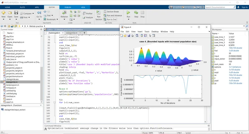
Output :-

Explaination of code :-

The Program starts with basic commands clear all, close all, clc

clear all- It is used to clear the data stored in the workspace.

close all- It is used to close the plots and figures etc.

clc- It is used to clear the command window.

First of all x and y arrays are defined and 150 equally spaced values between 0 to 0.6 are created using linspace command and these values are assigned to the x and y arrays.

Two dimensional mesh is created using meshgrid command and it is assigned to the xx and yy. Number of iteration of code is defined. It is given by 'num_cases=30'.

To evaluate values from stalagmite function nested for loop is used. 'i' vector is initialize and for every value of i vector separate 'j' vector is initialize using for loop.

Input vector variables are defined for xx and yy values, these are the inputs of stalagmite function.

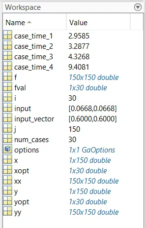
Tic-Toc command is used to know the time taken to solve the loop of 30 iterations. it is used before and after of each loop.

To obtain global maxima for each cases inbuilt 'ga' function is used. In the first case bounds are not defined and the plots are made using 'surfc' command.

shading interp command is used to avoid meshing line and to obtain smooth plot. subplot command is used to plot more than one plot in single window.

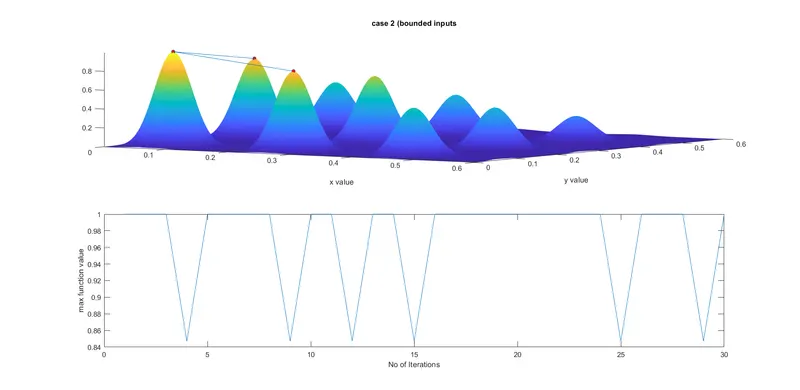
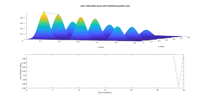
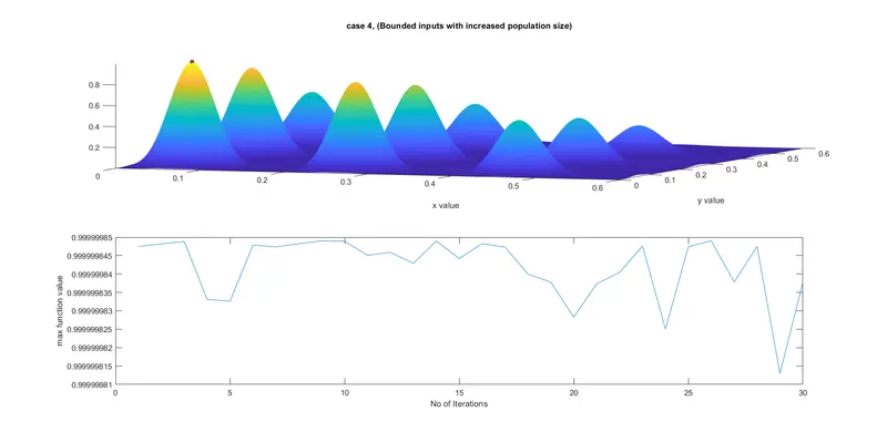
To obtain more accuracy bounding is given in the next cases as well as the population has been increased to obtain accurate values.

In this way the global maxima is found in the fourth case.

Output Plots :-

Case :- 1 (UnBounded)

l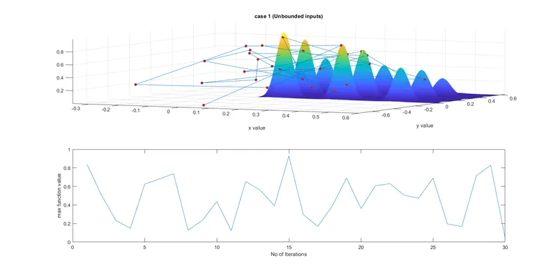

Case :- 2 (Bounded)

Case :- 3 (Bounded with modified population size)

Case :- 4 (Bounded with increased population size)

Workspace values :-

Conclusion :-

Thus we can conclude that Genetic algorithm gives more accurate results in case of bounded inputs and by increasing the population size and number of iterations.

References :-

https://www.mathworks.com/discovery/genetic-algorithm.html

https://en.wikipedia.org/wiki/Genetic_algorithm