Challenge

Project 2 - Rankine cycle Simulator

SSarang Vispute3 May 2022

Aim :- To write a program in MATLAB to create a Rankine Cycle Simulator.

Objective :-

To write a code to calculate all the state points of the cycle based on user inputs and simulate a Rankine cycle.
To plot the T-S and H-S diagrams for the given set of inputs.

Theory :-

The Rankine cycle is an idealized thermodynamic cycle. Rankine cycle is named after William John Macquorn Rankine, a Scottish polymath professor at Glasgow University. The Rankine cycle is the fundamental operating cycle of all power plants where an operating fluid is continuously evaporated and condensed. In this mechanism, a fuel is used to produce heat within a boiler, converting water into steam which then expands through a turbine producing useful work. The efficiency of the Rankine cycle is limited by the high heat of vaporization by the fluid. The fluid must be cycled through and reused constantly, therefore, water is the most practical fluid for this cycle.

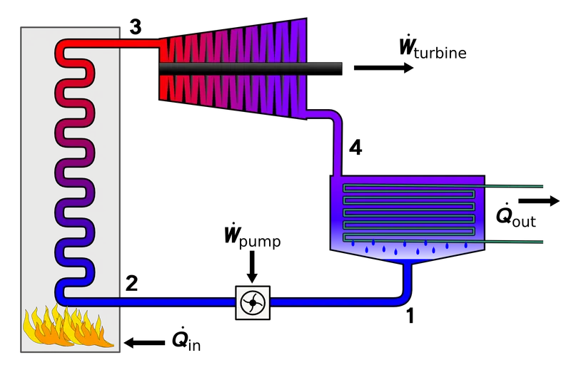
Rankine engines generally operate in a closed loop where the working fluid is reused. Heat energy is supplied to the system via a boiler where the working fluid (typically water) is converted to a high pressure gaseous state (steam) in order to turn a turbine. After passing over the turbine the fluid is allowed to condense back into a liquid state as waste heat energy is rejected before being returned to boiler.

Process 1–2: The working fluid is pumped from low to high pressure. As the fluid is a liquid at this stage, the pump requires little input energy. Process 1-2 is isentropic compression.
Process 2–3: The high-pressure liquid enters a boiler, where it is heated at constant pressure by an external heat source to become a dry saturated vapour. The input energy required can be easily calculated graphically, using an enthalpy–entropy chart(h–s chart, or Mollier diagram), or numerically, using steam tables or software. Process 2-3 is constant pressure heat addition in boiler.
Process 3–4: The dry saturated vapour expands through a turbine, generating power. This decreases the temperature and pressure of the vapour, and some condensation may occur. The output in this process can be easily calculated using the chart or tables noted above. Process 3-4 is isentropic expansion.
Process 4–1: The wet vapour then enters a condenser, where it is condensed at a constant pressure to become a saturated liquid. Process 4-1 is constant pressure heat rejection in condenser.

Program :-

clear all
close all
clc

%Rankine cycle simulator
disp('Rankine cycle')
disp('1-2 is Isentropic expansion in Turbine')
disp('2-3 is constant pressure heat rejection')
disp('3-4 is Isentropic compression in pump')
disp('4-1 is constant pressure heat addition')

%Input data
p1=input('\nEnter the value of pressure at turbine inlet, p1 (in bar) = ');
T1=input('Enter the value of temperature at turbine inlet, T1(in degree celcius) = ');
p2=input('Enter the value of pressure at condenser inlet, p2 (in bar) = ');

%Extracting data from Xsteam file
%State point 1
h1=XSteam('h_pT',p1,T1);
s1=XSteam('s_pT',p1,T1);

%State point 2
s2=s1;
sf2=XSteam('sL_p',p2);
sg2=XSteam('sV_p',p2);
x2=(s2-sf2)/(sg2-sf2);
hf2=XSteam('hL_p',p2);
hg2=XSteam('hV_p',p2);
h2=hf2+(x2*(hg2-hf2));


%State point 3
p3=p2;
s3=XSteam('sL_p',p3);
h3=XSteam('hL_p',p3);


%State point 4
s4=s3;
p4=p1;

%Work done by turbine
Wt=h1-h2;

%Work required to run the pump
v3=XSteam('vL_p',p3);
Wp=v3*(p4-p3)*100;
h4=h3+Wp;

%Net work
Wnet=Wt-Wp;

%Heat input in the system
Qin=h1-h4;

%heat exhaust from the system
Qout=h2-h3;

%Thermal efficiency
eff= (Wnet/Qin)*100;

%Specific heat consumption (mass flow rate/power)
SSC=(3600/Wnet);

%Calculation of teperature at all state points
T3=XSteam('Tsat_p',p3);
T2=T3;
Cp4=XSteam('Cp_ps',p4,s4);
Cv4=XSteam('Cv_ps',p4,s4);
k=Cp4/Cv4;
T4=T3/((p3/p4)^((k-1)/k));

%state points at liquid line
T6=XSteam('Tsat_p',p1);
s5=XSteam('sL_p',p1);
s6=XSteam('sv_p',p1);
h5=XSteam('hL_p',p1);
h6=XSteam('hV_p',p1);
T5=T6;

%Saturation curve
T=linspace(1,375,1000);
for i=1:length(T)
    sf(i)=XSteam('sL_T',T(i));
    sg(i)=XSteam('sV_T',T(i));
    hf(i)=XSteam('hL_T',T(i));
    hg(i)=XSteam('hV_T',T(i));
end

%Plotting T-S diagram
figure(1)
hold on
plot(sf,T,'color','r','linewidth',2);
plot(sg,T,'color','r','linewidth',2);
plot([s1 s2],[T1 T2],'color','b','linewidth',2);
plot([s2 s3],[T2 T3],'color','b','linewidth',2);
plot([s3 s4],[T3 T4],'color','b','linewidth',2);
plot([s4 s5],[T4 T5],'color','b','linewidth',2);
plot([s5 s6],[T5 T6],'color','b','linewidth',2);

sc1=linspace(s6,s1,1000);
for l=1:length(sc1)
    Tc1(l)=XSteam('T_ps',p1,sc1(l));
end
plot(sc1,Tc1,'color','b','linewidth',2)
text(s1+0.1,T1,'1')
text(s2+0.1,T2,'2')
text(s3,T3-20,'3')
text(s4,T4+20,'4')
title('Temperature vs Entropy (T-S Diagram)')
xlabel('\bf Entropy (S) [kj/kgk]')
ylabel('\bf Temperature (T) [degree c]')
legend ('Saturation curve')

%Plotting h-s diagram
figure(2)
hold on
plot(sf,hf,'color','r','linewidth',2);
plot(sg,hg,'color','r','linewidth',2);
plot([s1 s2],[h1 h2],'color','b','linewidth',2);
plot([s2 s3],[h2 h3],'color','b','linewidth',2);
plot([s3 s4],[h3 h4],'color','b','linewidth',2);
hc=linspace(h4,h5,100);
for k=1:length(hc)
sch(k)=XSteam('s_ph',p1,hc(k));
end
plot(sch,hc,'color','b','linewidth',2);
plot([s5 s6],[h5 h6],'color','b','linewidth',2);
for m=1:length(sc1)
    hc1(m)=XSteam('h_ps',p1,sc1(m));
end
plot(sc1,hc1,'color','b','linewidth',2);
text(s1+0.1,h1,'1')
text(s1+0.1,h2,'2')
text(s3,h3-100,'3')
text(s4,h4+200,'4')
title('Enthalpy vs Entropy (H-S Diagram)')
xlabel('\bfEntropy (S) [kj/kgk]')
ylabel('\bfEnthalpy (H) [kj/kg]')
legend ('Saturation curve')

%Results 
disp('Results')
fprintf('At State point 1:-')
fprintf('\np1: %.3f bar',p1);
fprintf('\nT1: %.3f C',T1);
fprintf('\nh1: %.3f kj/kg',h1);
fprintf('\ns1: %.3f kj/kgk',s1);
fprintf('\n\nAt State point 2:-')
fprintf('\np2: %.3f bar',p2);
fprintf('\nT2: %.3f C',T2);
fprintf('\nh2: %.3f kj/kg',h2);
fprintf('\ns2: %.3f kj/kgk',s2);
fprintf('\nx2: %.3f',x2);
fprintf('\n\nAt State point 3:-');
fprintf('\np3: %.3f bar',p3);
fprintf('\nT3: %.3f C',T3);
fprintf('\nh3: %.3f kj/kg',h3);
fprintf('\ns3: %.3f kj/kgk',s3);
fprintf('\n\nAt State point 4:-');
fprintf('\np4: %.3f bar',p4);
fprintf('\nT4: %.3f C',T4);
fprintf('\nh4: %.3f kj/kg',h4);
fprintf('\ns4: %.3f kj/kgk',s4);
fprintf('\n\nTurbine Work: %.3f kj/kg',Wt);
fprintf('\nPump Work: %.3f kj/kg',Wp);
fprintf('\nWnet: %.3f kj/kg',Wnet);
fprintf('\nEfficiency: %.3f Percent ',eff);
fprintf('\nSSC: %.3f kj/kWh',SSC)

Output :-

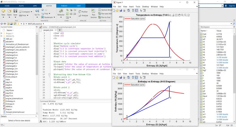
Explaination of code :-

The Program starts with basic commands clear all, close all, clc

clear all- It is used to clear the data stored in the workspace.

close all- It is used to close the plots and figures etc.

clc- It is used to clear the command window.

First of all all four processes are displayed in command window using 'disp' command.

Input values of P1, T1, P2 are required to enter in the command window while executing the program.

XSteam data is used to extract the steam and water properties of temperature, enthalpy, entropy, specific pressure for saturated liquid and saturated vapour conditions.

To extract the values from XSteam data it is required to use this default syntax h1=XSteam('h_pT', p1, t1) It extracts the enthalpy of water at given pressure and temperature. similarly all the variables for all states are extracted using this format.

After extraction of all values we have used standard Thermodynamic formula to calculate the Net work (wnet=Wt-Wp), Thermal efficiency and specific heat consumption.

the values of temperature and state points at liquid line are extracted from XSteam data.

The values of sf, sg, hf ,hg are calculated where f and g stands for saturated liquid and saturated vapour respectively for saturation curve.

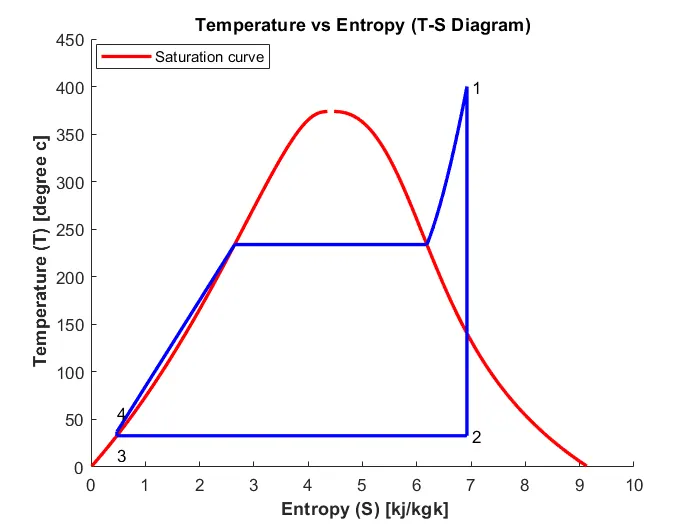
The graph of Temperature vs Entropy is plotted using plot command. saturaction curve is also plotted and represented by red colur.

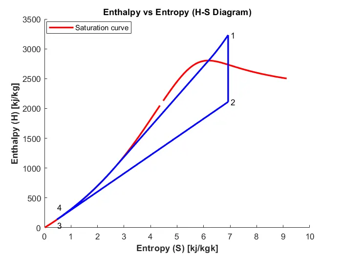
As well as the graph of Enthalpy vs Entropy is plotted using plot command and labels are displayed on x axis and y axis using 'xlabel' and 'ylabel' commands respectively.

All the results are displayed in the command window using 'fprintf' command.

Results :-

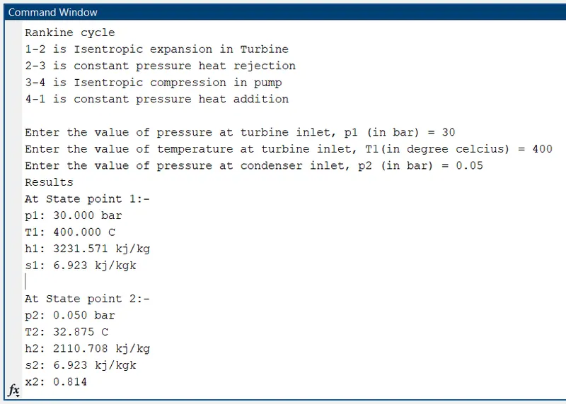
Rankine cycle
1-2 is Isentropic expansion in Turbine
2-3 is constant pressure heat rejection
3-4 is Isentropic compression in pump
4-1 is constant pressure heat addition

Enter the value of pressure at turbine inlet, p1 (in bar) = 30
Enter the value of temperature at turbine inlet, T1(in degree celcius) = 400
Enter the value of pressure at condenser inlet, p2 (in bar) = 0.05
Results
At State point 1:-
p1: 30.000 bar
T1: 400.000 C
h1: 3231.571 kj/kg
s1: 6.923 kj/kgk

At State point 2:-
p2: 0.050 bar
T2: 32.875 C
h2: 2110.708 kj/kg
s2: 6.923 kj/kgk
x2: 0.814

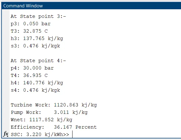
At State point 3:-
p3: 0.050 bar
T3: 32.875 C
h3: 137.765 kj/kg
s3: 0.476 kj/kgk

At State point 4:-
p4: 30.000 bar
T4: 36.935 C
h4: 140.776 kj/kg
s4: 0.476 kj/kgk

Turbine Work: 1120.863 kj/kg
Pump Work:    3.011 kj/kg
Wnet: 1117.852 kj/kg
Efficiency:   36.167 Percent 
SSC: 3.220 kj/kWh>>

Output Plots :-

T-S diagram :-