Week 4.1 - Genetic Algorithm

AIM : To optimise the stalagmite function and find the global maxima of the function

OBJECTIVE OF THE PROJECT:

• Write a code in MATLAB to optimise the stalagmite function and find the global maxima of the function.
• Clearly expalin the concept of genetic algorithm in your own words and also explain the syntax for ga in MATLAB in your report.
• Make sure that your code gives the same output, even if it is made to run several times.
• Plot graphs for all 3 studies and for F maximum vs no. of iterations. Title and axes labels are a must, legends could be shown if necessary

THEORY OF GA:

A genetic algorithm is a search heuristic that is inspired by Charles Darwin’s theory of natural evolution. This algorithm reflects the process of natural selection where the fittest individuals are selected for reproduction in order to produce offspring of the next generation.

NATION OF NATURAL SELECTION

The process of natural selection starts with the selection of fittest individuals from a population. They produce offspring which inherit the characteristics of the parents and will be added to the next generation. If parents have better fitness, their offspring will be better than parents and have a better chance at surviving. This process keeps on iterating and at the end, a generation with the fittest individuals will be found.

This notion can be applied for a search problem. We consider a set of solutions for a problem and select the set of best ones out of them.

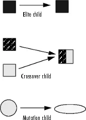
Five phases are considered in a genetic algorithm.

1. Initial population
2. Fitness function
3. Selection
4. Crossover
5. Mutation

Initialization of population (coding):

The population size depends on the nature of the problem, but typically contains several hundreds or thousands of possible solutions. Often, the initial population is generated randomly, allowing the entire range of possible solutions (the search space). Occasionally, the solutions may be "seeded" in areas where optimal solutions are likely to be found.

Fitness function:

The fitness function determines how fit an individual is (the ability of an individual to compete with other individuals). It gives a fitness score to each individual. The probability that an individual will be selected for reproduction is based on its fitness score.

Selection:

The idea of selection phase is to select the fittest individuals and let them pass their genes to the next generation.

Two pairs of individuals (parents) are selected based on their fitness scores. Individuals with high fitness have more chance to be selected for reproduction.

Crossover:

Crossover is the most significant phase in a genetic algorithm. For each pair of parents to be mated, a crossover point is chosen at random from within the genes.

Mutation

In certain new offspring formed, some of their genes can be subjected to a mutation with a low random probability. This implies that some of the bits in the bit string can be flipped.

FLOW CHART:

SYNTEX FOR GA:

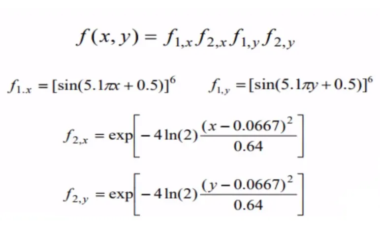
• the above equation is used in the stalagmite function to plot the graph in the main function.

FUNCTION CODE:

function[F]=stalagmite(input_vector)

x = input_vector(1);
y = input_vector(2);

f1_x = (sin(5.1*pi*x+0.5))^6;
f1_y = (sin(5.1*pi*y+0.5))^6;

p1 = (x-0.0667)^2/0.64;
f2_x = exp(-4*log(2)*p1);

p2 = (y-0.0667)^2/0.64;
f2_y=exp(-4*log(2)*p2);

F = -(f1_x.*f2_x.*f1_y.*f2_y);

end

• while using the function at the end of the line we use -ve sign because the plot will come reverse to find the maxima using GA.

PROGRAM:

without boundation

close all
clear all
clc


% Defining our search space for the function
x = linspace(0,0.6,150);
y = linspace(0,0.6,150);
num_case = 50; % iteration count is 50 that means GA runs for 50 iteration

% For creating 2D array

[xx, yy] = meshgrid(x,y);

% Evaluating the stalagmite function
for i = 1:length(xx)
    for j = 1:length(yy)
        input_vector(1) = xx(i,j);
        input_vector(2) = yy(i,j);
        f(i,j)=stalagmite(input_vector);

    end
end
surfc(xx,yy,-f)
xlabel('x_value')
ylabel('y_value')
shading interp

RESULTS:

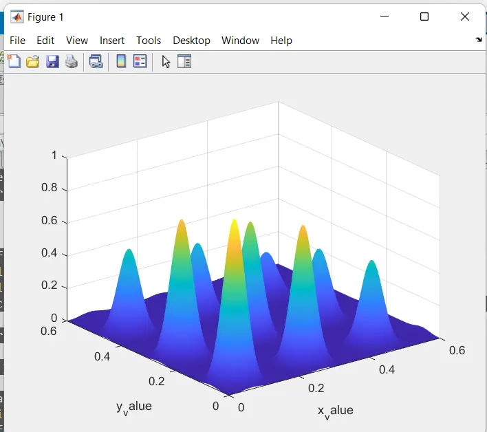
EXPLAINATION:

• Here first start the program with 'close all','clear all','clc'.
• And we define the 2 variable which is act as serch space to find the global maxima.
• we give num case value for iteration of ga so that it will give optimum value.
• create it in 2d array using meshgrid.
• now calculating the value of fitness function at each point of mesh grid formed.
• now creating the plot using surfc command which will also provide countour of the generated surface
• while using surfc we give -ve sign for the function so it shows upward.
• we use shading interp command so that the plot will look smooth without mesh.

STATICAL STUDY WIYHOIUT BOUNDATION

%% STATISTICAL BEHAVIOUR (UNBOUNDED)
tic % Study time count start
for i =1:num_case
    [inputs, fval(i)] = ga(@stalagmite, 2); % GA function runs the stalagmite data and gives the optimal solution
  x_opt(i) = inputs(1);
  y_opt(i) = inputs(2);

end
study1_time = toc; % Stuty time count end

figure(2)
subplot(2,1,1)
hold on
surfc(xx,yy,-f) % Generating stalagmite function
shading interp % for smooth curve without mesh grid
plot3(x_opt,y_opt,-fval,'marker','o','MarkerSize',4,'MarkerFaceColor','r') % Plotting the optimum value with a red dot marker along the stalagmite 3D curves
title('unbounded inputs')

subplot(2,1,2)
plot(-fval)  % Plot of opt_f for every iterations
xlabel('number of iterations')
ylabel('function max')

RESULT

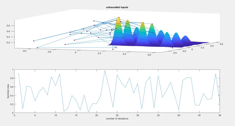
EXPLAINAION:

• Here we give tic and toc for the count of study time of optimization.
• we use above syntex here to find the optimm value of fitness function(which gives the inputs i.e; get value of x and y for the minimum of the function).
• then plot using surfc and also give the optimum values of the function how it is variying.

Conclusion:

• here we get a lots of variation and difficult to get a maxima value

statastical study with boundation

%% STATISICAL BEHAVIOUR (BOUNDED)

tic % Study time count start 
for j = 1:num_case
    % Objective function is stalagmite and the no of variable is 2
    % A,B,Aeq and Beq = [] as their is no linear equalities and inequalities constrains in this function
    % Lower bountries of variable x and y in ga algorithm is set as [0,0]
    % Upper bountries of variable x and y in ga algorithm is set as [0.6,0.6]
     [inputs, fval(j)] = ga(@stalagmite, 2,[],[],[],[],[0,0],[0.6,0.6]); % GA function runs the stalagmite data and gives the optimal solution
     x_opt(j) = inputs(1);
     y_opt(j) = inputs(2);

end
study2_time = toc; % Stuty time count end

figure(3)
subplot(2,1,1)
hold on
surfc(xx,yy,-f) % Generating stalagmite function
shading interp % for smooth curve without mesh grid
plot3(x_opt,y_opt,-fval,'marker','o','MarkerSize',5,'MarkerFaceColor','r') % Plotting the optimum value with a red dot marker along the stalagmite 3D curves
title('bounded inputs')
subplot(2,1,2)
plot(-fval)  % Plot of opt_f for every iterations
xlabel('number of iterations')
ylabel('function max')

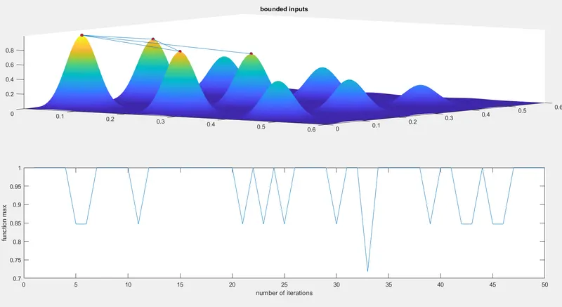
RESULTS:

EXPLAINATION:

• Here everything is same as avobe we just provide the upper bound and lower bound to ga so get the serch space is reduced with lower and upper limits.
• And plotting is similar as above study.

CONCLUSION:

• It is clear that from the above study after providing the lmits the variation is reduced but not as much clear.

STATISTICAL STUDY BY INCREASING THE SIZE OF POPULATION

%% MODIFYING THE NUMBER OF POPULATION
options = optimoptions('ga');
options = optimoptions(options,'PopulationSize',200);
tic %study time start
for k = 1:num_case
     [inputs, fval(k)] = ga(@stalagmite, 2,[],[],[],[],[0,0],[0.6,0.6],[],options); % GA function runs the stalagmite data and gives the optimal solution
  x_opt(k) = inputs(1);
  y_opt(k) = inputs(2);

end
study3_time = toc % Stuty time count end

figure(4)
subplot(2,1,1)
hold on
surfc(xx,yy,-f) % Generating stalagmite function
shading interp % for smooth curve without mesh grid
plot3(x_opt,y_opt,-fval,'marker','o','MarkerSize',4,'MarkerFaceColor','r') % Plotting the optimum value with a red dot marker along the stalagmite 3D curves

subplot(2,1,2)
plot(-fval)  % Plot of opt_f for every iterations
xlabel('number of iterations')
ylabel('function max')

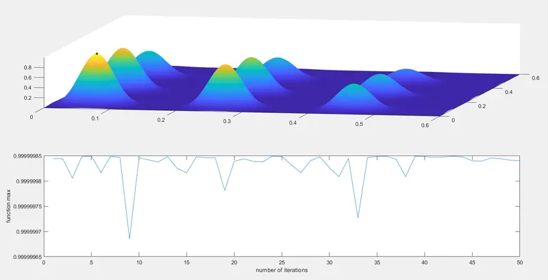
RESULT:

EXPLAINATION:

• Here we use the 'optimoptions' command to increase the size of population so that it will give much better result for the fitness of function.
• Here is a drawback that it take a lot time to optimize.

CONCLUSION:

• Here we can clearly see that in above case that the result various is improved.

NOW THE WHOLE PROGRAM AT ONCE

close all
clear all
clc


% Defining our search space for the function
x = linspace(0,0.6,150);
y = linspace(0,0.6,150);
num_case = 50; % iteration count is 50 that means GA runs for 50 iteration

% For creating 2D array

[xx, yy] = meshgrid(x,y);

% Evaluating the stalagmite function
for i = 1:length(xx)
    for j = 1:length(yy)
        input_vector(1) = xx(i,j);
        input_vector(2) = yy(i,j);
        f(i,j)=stalagmite(input_vector);

    end
end
surf(xx,yy,-f)
xlabel('x_value')
ylabel('y_value')
shading interp
%% STATISTICAL BEHAVIOUR (UNBOUNDED)
tic % Study time count start
for i =1:num_case
    [inputs, fval(i)] = ga(@stalagmite, 2); % GA function runs the stalagmite data and gives the optimal solution
  x_opt(i) = inputs(1);
  y_opt(i) = inputs(2);

end
study1_time = toc; % Stuty time count end

figure(2)
subplot(2,1,1)
hold on
surfc(xx,yy,-f) % Generating stalagmite function
shading interp % for smooth curve without mesh grid
plot3(x_opt,y_opt,-fval,'marker','o','MarkerSize',4,'MarkerFaceColor','r') % Plotting the optimum value with a red dot marker along the stalagmite 3D curves
title('unbounded inputs')

subplot(2,1,2)
plot(-fval)  % Plot of opt_f for every iterations
xlabel('number of iterations')
ylabel('function max')
%% STATISICAL BEHAVIOUR (BOUNDED)

tic % Study time count start 
for j = 1:num_case
    % Objective function is stalagmite and the no of variable is 2
    % A,B,Aeq and Beq = [] as their is no linear equalities and inequalities constrains in this function
    % Lower bountries of variable x and y in ga algorithm is set as [0,0]
    % Upper bountries of variable x and y in ga algorithm is set as [0.6,0.6]
     [inputs, fval(j)] = ga(@stalagmite, 2,[],[],[],[],[0,0],[0.6,0.6]); % GA function runs the stalagmite data and gives the optimal solution
     x_opt(j) = inputs(1);
     y_opt(j) = inputs(2);

end
study2_time = toc; % Stuty time count end

figure(3)
subplot(2,1,1)
hold on
surfc(xx,yy,-f) % Generating stalagmite function
shading interp % for smooth curve without mesh grid
plot3(x_opt,y_opt,-fval,'marker','o','MarkerSize',5,'MarkerFaceColor','r') % Plotting the optimum value with a red dot marker along the stalagmite 3D curves
title('bounded inputs')
subplot(2,1,2)
plot(-fval)  % Plot of opt_f for every iterations
xlabel('number of iterations')
ylabel('function max')

%% MODIFYING THE NUMBER OF POPULATION
options = optimoptions('ga');
options = optimoptions(options,'PopulationSize',200);
tic %study time start
for k = 1:num_case
     [inputs, fval(k)] = ga(@stalagmite, 2,[],[],[],[],[0,0],[0.6,0.6],[],options); % GA function runs the stalagmite data and gives the optimal solution
  x_opt(k) = inputs(1);
  y_opt(k) = inputs(2);

end
study3_time = toc % Stuty time count end

figure(4)
subplot(2,1,1)
hold on
surfc(xx,yy,-f) % Generating stalagmite function
shading interp % for smooth curve without mesh grid
plot3(x_opt,y_opt,-fval,'marker','o','MarkerSize',4,'MarkerFaceColor','r') % Plotting the optimum value with a red dot marker along the stalagmite 3D curves

subplot(2,1,2)
plot(-fval)  % Plot of opt_f for every iterations
xlabel('number of iterations')
ylabel('function max')