Week 3 - Solving second order ODEs
AIM: To solve second order ordinary differencial equation using matlab
THEORY :
an ordinary differential equation (ODE) is a differential equation containing one or more functions of one independent variable and the derivatives of those functions. The term ordinary is used in contrast with the term partial differential equation which may be with respect to more than one independent variable.
Simple pendulum
The simple pendulum is another mechanical system that moves in an oscillatory motion. It consists of a point mass ‘m’ suspended by means of light inextensible string of length L from a fixed support as shown in Fig. 2.8. The motion occurs in a vertical plane and is driven by a gravitational force. The forces which are acting on the mass are shown in the figure. The tangential component of the gravitational force, mg sin θ, always acts towards the mean position θ = 0 opposite to the displacement, restoring force acting tangent to the arc.
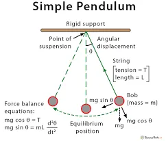
GOVERNING EQUATION:
now we have to breake it into single order equation
let us consider
theta = theta1 --------- (1)
dtheta/dt = dtheta1/dt = theta2 --------(2)
d^2theta/dt^2 = dtheta2/dt --------(3)
- by using these 3 equation we have
dtheta2/dt = -b/m*theta2 - g/l*sintheta1
PROGRAM:
Function Program
function [dtheta_dt] = ode_func(t,theta,b,g,l,m)

theta1 = theta(1);
theta2 = theta(2);
dtheta1_dt = theta2;
dtheta2_dt = -(b/m)*theta2 - (g/l)*sin(theta1);
dtheta_dt = [dtheta1_dt;dtheta2_dt];

end
Main Program
clear all
close all
clc

% Inputs variable
b = 0.05;            % damping coefficient
g = 9.81;            %gravitational acceleration in m/s^2
l = 1;               %length in metre
m = 1;               % mass in kilograms

% Initial conditions
theta_0 = [0;5];

% time point
t_span = linspace(0,10,500);

%solve ODE
[t,results] = ode45(@(t,theta) ode_func(t,theta,b,g,l,m), t_span, theta_0);

plot(t,results(:,1));
hold on
plot(t,results(:,2));
xlabel('time')
ylabel('point')

figure(2)
ct = 1;
for i=1:length(results(:,1))

    % fixed coordinates at one end
    x0 = 0;
    y0= 0;

    x1 = l*sin(results(i,1));
    y1 = -l*cos(results(i,1));

    %plotting of fixed side
    plot([-1 1],[0 0],'linewidth',3,'color','b')
    hold on
    plot([x0 x1],[y0 y1],'linewidth',3,'Color','g')
    plot(x1,y1,'marker','o','markersize',30,'color','r')
    axis([-1.5 2 -1.5 2])
    pause(0.003)

%creating movie
M(ct) = getframe(gcf);
hold off
ct = ct+1;
end

videofile = VideoWriter("simple_pendulum.avi","uncompressed AVI");
open(videofile)
writeVideo(videofile,M);
close(videofile);
CODE EXPLAINATION:
- Start the program with
close all(close all the previous data and file)
clear all (clear the previous files)
clc(clear the command window)
- give the comment %input variable and give inputs
give the value of b,g,l,m
- giving %initial conditions from where the displacement and velocity starts
- now solve the ODE using 'ODE45' code in matlab following the function
[t,results] = ode45(@(t,theta) ode_func(t,theta,b,g,l,m), t_span, theta_0)
- plot the (displacement,velocity) with respect to time graph using 'plot' graph
- giving 'xlebel' & 'ylebel'
- for creating animation of simple pendulum we are going to use for loop
- inside the for loop we are are going to put the value of coordinate as "x0,y0,x1,y2"
- and by using that cordinate we are going to plot the pendulum in movie
- and use the axis and also pause command
- and now we are going to give the movie formate as follows
M(ct) = getframe(gcf) [for getting all that into a frame]
videofile = VideoWriter("simple_pendulum.avi","uncompressed AVI") [give the file name and formate of file]
open(videofile) [open the video file writeVideo(videofile,M) [write the video file and M] close(videofile) [close the video file]
RESULTS:
youtube link: https://youtu.be/MYHTT4f8WQM