Week 4.1 - Genetic Algorithm

Genetic Algorithm

AIM:-

1. To write a code in MATLAB to optimise the stalagmite function and find the global maxima of the function.
2. To clearly explain the concept of genetic algorithm and also to explain the syntax for ga in MATLAB.
3. To make sure that code gives the same output, even if it is made to run several times.
4. To plot graphs for all case studies and for F maximum vs no. of iterations.

Principle:- In order to understand the concept of the Genetic algorithm, first we should understand the Optimisation process.

Optimisation is a decision making process, it helps to find the best results under a set of prioritised criteria or constraints. It is a procedure which is executed iteratively by comparing various solutions till an optimum or a satisfactory solution is found. These include maximising factors such as productivity, strength, reliability, efficiency, etc. Optimisation is the act of changing an existing process in order to increase the occurrence of favourable outcomes and decrease the occurrence of undesirable outcomes. Optimization is the discipline of adjusting a process so as to optimise (make the best or most effective use of) some specified set of parameters without violating some constraint. The most common goals are minimising cost and maximising throughput and/or efficiency. This is one of the major quantitative tools in industrial decision making.

The following is the procedure followed by any optimisation process:

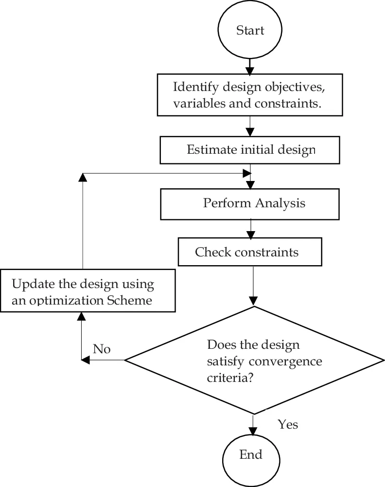
Figure 1: Flow chart of Optimisation process.

The parameters which have to vary during the optimisation process are known as variables. Design dimensions can be varied to get the minimum stress. During the optimisation process output should not go beyond the certain limits, those are known as constraints. Objective function is as simple as a mathematical formulae, which can be a predicted mathematical model that includes all the variables as input. Let’s take z = f(x, y), here the outputs depends on the input variable(x and y). The variable bounds are the range of the input variables, that will be varied for every iteration to provide an optimised result. The design variable (thickness) can be varied in the range between (5-7)mm, to get the minimum stress.

Example : Let’s take designing a simply supported beam to withstand the load of 1-tonne, in tis case you need to consider the following parameters: length, breadth, width, factor of safety, weight and stress induced, here optimisation helps to find the best value for length, breadth and width of the beam in such a way that the factor of safety, material consumed and stress induced are within the limit.

We need to choose an optimisation algorithm to perform the optimisation process. Genetic algorithm is one of the optimisation processes.

Genetic Algorithm (GA) is a search based optimisation technique based on the principles of Genetics and Natural selection. It is frequently used to find optimal or near optimal solutions. It is frequently used to solve optimisation problems, in research, and in machine learning. The genetic algorithm is a method for solving both constrained and unconstrained optimisation problems that is based on natural selection, the process that drives biological evolution. The genetic algorithm repeatedly modifies a population of individual solutions.

At each step, the genetic algorithm selects individuals from the current population to be parents and uses them to produce the children for the next generation. Over successive generations, the population "evolves" toward an optimal solution. You can apply the genetic algorithm to solve a variety of optimisation problems that are not well suited for standard optimisation algorithms, including problems in which the objective function is discontinuous, non differentiable or highly nonlinear.

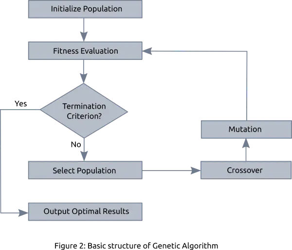
The process of natural selection starts with the selection of fittest individuals from a population. They produce offspring which inherit the characteristics of the parents and will be added to the next generation. If parents have better fitness, their offspring will be better than parents and have a better chance at surviving. This process keeps on iterating and at the end, a generation with the fittest individuals will be found. This notion can be applied for a search problem. We consider a set of solutions for a problem and select the set of best ones out of them.

Five phases are considered in a genetic algorithm.

1. Initial population
2. Fitness function
3. Selection
4. Crossover
5. Mutation

• Initial Population - The process begins with a set of individuals which is called a Population. Each individual is a solution to the problem you want to solve. An individual is characterised by a set of parameters (variables) known as Genes. Genes are joined into a string to form a Chromosome (solution). The population size depends on the nature of the problem, but typically contains several hundreds or thousands of possible solutions. Often, the initial population is generated randomly, allowing the entire range of possible solutions (the search space). Occasionally, the solutions may be "seeded" in areas where optimal solutions are likely to be found.

• Fitness Function - The fitness function determines how fit an individual is (the ability of an individual to compete with other individuals). It gives a fitness score to each individual. The probability that an individual will be selected for reproduction is based on its fitness score. It is a function which measures how good solution is. Fitness function takes the solution as input and produces the suitability of the solution as the output. This evaluates how close the solution is to the optimal solution of the desired problem.

• Selection - The idea of selection phase is to select the fittest individuals and let them pass their genes to the next generation. Two pairs of individuals (parents) are selected based on their fitness scores. Individuals with high fitness have more chance to be selected for reproduction. During each successive generation, a portion of the existing population is selected to breed a new generation. Individual solutions are selected through a fitness-based process, where fitter solutions (as measured by a fitness function) are typically more likely to be selected. Certain selection methods rate the fitness of each solution and preferentially select the best solutions. Other methods rate only a random sample of the population, as the former process may be very time-consuming.

• Crossover - It is the process of taking two parents and producing the Childs from them by interchanging the genes. Crossover is the most significant phase in a genetic algorithm. For each pair of parents to be mated, a crossover point is chosen at random from within the genes. Offspring are created by exchanging the genes of parents among themselves until the crossover point is reached. The new offspring are added to the population.

• Mutation - Mutation is carried out to maintain the genetic diversity from one generation of a population of chromosomes to the next. In this process, the genes will be replaced by some random integers. In certain new offspring formed, some of their genes can be subjected to a mutation with a low random probability. This implies that some of the bits in the bit string can be flipped. Mutation occurs to maintain diversity within the population and prevent premature convergence. If mutation is not performed, the chromosomes will become too similar to each other, convergence takes place soon and results in local minima.

• Termination - The algorithm terminates if the population has converged (does not produce offspring which are significantly different from the previous generation). Then it is said that the genetic algorithm has provided a set of solutions to our problem.

The termination condition of a Genetic Algorithm is important in determining when a GA run will end. It has been observed that, initially, the GA progresses very fast with better solutions coming in every few iterations, but this tends to saturate in the later stages where the improvements are very small. We usually want a termination condition such that our solution is close to the optimal, at the end of the run. One of the following termination conditions are:

• When there has been no improvements in the population for n number of generations.
• When we reach an absolute number of generations.
• When the objective function value has been reached a certain predefined value.

Genetic Algorithms are primarily used in optimisation problems of various kinds, but they are frequently used in other application areas as well. In this section, we list some of the areas in which Genetic Algorithms are frequently used. These are −

• Optimization − Genetic Algorithms are most commonly used in optimisation problems wherein we have to maximise or minimise a given objective function value under a given set of constraints. The approach to solve Optimization problems has been highlighted throughout the tutorial.
• Image Processing − GAs are used for various digital image processing (DIP) tasks as well like dense pixel matching.
• Vehicle routing problems − With multiple soft time windows, multiple depots and a heterogeneous fleet.
• Scheduling applications − GAs are used to solve various scheduling problems as well, particularly the time tabling problem.
• Machine Learning − as already discussed, genetics based machine learning (GBML) is a niche area in machine learning.
• Robot Trajectory Generation − GAs have been used to plan the path which a robot arm takes by moving from one point to another.
• Parametric Design of Aircraft − GAs have been used to design aircrafts by varying the parameters and evolving better solutions.
• Traveling salesman problem and its applications − GAs have been used to solve the TSP, which is a well-known combinatorial problem using novel crossover and packing strategies.

Genetic Algorithm (GA) Syntax:- Find minimum of function using genetic algorithm.

• x = ga(fun, nvars, A, b, Aeq, beq, lb, ub, nonlcon, intcon, options) -

• x = ga(fun, nvars) finds a local unconstrained minimum, x, to the objective function, fun. nvars is the dimension (number of design variables) of fun.
• x = ga(fun, nvars, A, b) finds a local minimum x to fun, subject to the linear inequalities A*x ≤ b. ga evaluates the matrix product A*x as if x is transposed (A*x').
• x = ga(fun, nvars, A, b, Aeq, beq) finds a local minimum x to fun, subject to the linear equalities Aeq*x = beq and A*x ≤ b. (Set A=[ ] and b=[ ] if no linear inequalities exist.) ga evaluates the matrix product Aeq*x as if x is transposed (Aeq*x').
• x = ga(fun, nvars, A, b, Aeq, beq, lb, ub) defines a set of lower and upper bounds on the design variables, x, so that a solution is found in the range lb ≤ x ≤ ub. (Set Aeq=[ ] and beq=[ ] if no linear equalities exist.)
• x = ga(fun, nvars, A, b, Aeq, beq, lb, ub, nonlcon) subjects the minimization to the constraints defined in nonlcon. The function nonlcon accepts x and returns vectors C and Ceq, representing the nonlinear inequalities and equalities respectively. ga minimizes the fun such that C(x) ≤ 0 and Ceq(x) = 0. (Set lb=[ ] and ub=[ ] if no bounds exist.)
• x = ga(fun, nvars, A, b, Aeq, beq, lb, ub, nonlcon, options) minimizes with the default optimization parameters replaced by values in options. (Set nonlcon=[ ] if no nonlinear constraints exist.) Create options using optimoptions.
• x = ga(fun, nvars, A, b, Aeq, beq, lb, ub, nonlcon, intcon) or x = ga(fun, nvars, A, b, Aeq, beq, lb, ub, nonlcon, intcon, options) requires that the variables listed in intcon take integer values.

When there are integer constraints, ga does not accept nonlinear equality constraints, only nonlinear inequality constraints.

• [x, fval, exitflag, output, population, scores] = ga(___) -

• [x, fval] = ga(___), for any previous input arguments, also returns fval, the value of the fitness function at x.
• [x, fval, exitflag, output] = ga(___) also returns exitflag, an integer identifying the reason the algorithm terminated, and output, a structure that contains output from each generation and other information about the performance of the algorithm.
• [x, fval, exitflag, output, population, scores] = ga(___) also returns a matrix population, whose rows are the final population, and a vector scores, the scores of the final population.

• options = optimoptions(SolverName, Name, Value) returns options with specified parameters set using one or more name-value pair arguments.

• surfc(X, Y, Z) creates a three-dimensional surface plot with a contour plot underneath. A surface plot is a three-dimensional surface that has solid edge colors and solid face colors. The function plots the values in matrix Z as heights above a grid in the x-y plane defined by X and Y. The color of the surface varies according to the heights specified by Z.

• subplot(m, n, p) divides the current figure into an m-by-n grid and creates axes in the position specified by p. MATLAB® numbers subplot positions by row. The first subplot is the first column of the first row, the second subplot is the second column of the first row, and so on. If axes exist in the specified position, then this command makes the axes the current axes.

• plot3(X, Y, Z) plots coordinates in 3-D space. To plot a set of coordinates connected by line segments, specify X, Y, and Z as vectors of the same length. To plot multiple sets of coordinates on the same set of axes, specify at least one of X, Y, or Z as a matrix and the others as vectors.

Stalagmite Function:- It is a kind of objective function as a mathematical formulae used in GA , which can be a predicted as mathematical model that includes all the variables as input, here the outputs depends on the input variable. The variable bounds are the range of the input variables, that will be varied for every iteration to provide an optimised result. Stalagmite function is a function on which GA is to operate to find function variable, global maxima.

Equation -

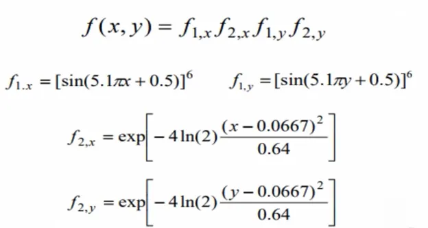
Figure 3: Equation of Satalgmite Function

Where,

x and y are the input variables.

Program:-

Initially stalagmite function code is generated based on the above mathematical formulae, explained under stalagmite function. Genetic Algorithm (ga) is going to operate on this function and need to find Global Maxima of the same.

function [f] = stalagmite(input)

f1x = (sin(5.1*pi*input(1) + 0.5)).^6;
f1y = (sin(5.1*pi*input(2) + 0.5)).^6;
f2x = exp(-4*log(2)*((input(1) - 0.0667).^2/(0.64)));
f2y = exp(-4*log(2)*((input(2) - 0.0667).^2/(0.64)));
f = -(f1x*f2x*f1y*f2y);

end

To optimise the stalagmite function and to find the global maxima of the function, below code is written,

% Optimization
 clear all
 close all
 clc

% Defining search space
 x = linspace(0, 0.6, 150);
 y = linspace(0, 0.6, 150);

% Creating 2Dimensional mesh
 [xx, yy] = meshgrid(x, y);

% Evaluating stalagmite function 
 for i = 1:length(xx)
  for j = 1:length(yy)
    input(1) = xx(i, j);
    input(2) = yy(i, j);
    f(i, j) = stalagmite(input);
  end
 end

% Genetic algorithm solver (ga)
[inputs0, fval0] = ga(@stalagmite, 2);

% Exploring 3 different cases of ga to get same global maxima value of the function every time the code is execute
% Case1
% no. of iterations
iteration = 50;

for i = 1: iteration
[inputs1, fval1(i)] = ga(@stalagmite, 2); 
xopt1(i) = inputs1(1);
yopt1(i) = inputs1(2);
end

% Plot graph to monitor solver progress
subplot(2, 1, 1)
surfc(xx, yy, -f)
shading interp
hold on
plot3(xopt1, yopt1, -fval1, 'Marker','o','MarkerSize',5,'MarkerFaceColor','r')
title('Case1 Unbounded statistical behaviour')
subplot(2, 1, 2)
plot(-fval1)
xlabel('no. of iterations')
ylabel('F maximum')

% Case2
% Set bounds lb(lowerbounds) and ub(upperbounds)
for i = 1: iteration
[inputs2, fval2(i)] = ga(@stalagmite, 2, [ ], [ ], [ ], [ ], [0,0], [0.6,0.6]); 
xopt2(i) = inputs2(1);
yopt2(i) = inputs2(2);
end

% Plot graph to monitor solver progress
figure(2)
subplot(2, 1, 1)
surfc(xx, yy, -f)
shading interp
hold on
plot3(xopt2, yopt2, -fval2, 'Marker','o','MarkerSize',5,'MarkerFaceColor','r')
title('Case2 Bounded statistical behaviour')
subplot(2, 1, 2)
plot(-fval2)
xlabel('no. of iterations')
ylabel('F maximum')

% Case3
% To obtain more accurate solution increasing options size by changing populationsize 
options = optimoptions('ga', 'PopulationSize', 250);

for i = 1: iteration
[inputs3, fval3(i)] = ga(@stalagmite, 2, [ ], [ ], [ ], [ ], [0,0], [0.6,0.6], [ ], [ ], options); 
xopt3(i) = inputs3(1);
yopt3(i) = inputs3(2);
end

% Plot graph to monitor solver progress
figure(3)
subplot(2, 1, 1)
surfc(xx, yy, -f)
shading interp
hold on
plot3(xopt3, yopt3, -fval3, 'Marker','o','MarkerSize',5,'MarkerFaceColor','r')
title('Case3 Bounded inputs with modified populationsize')
subplot(2, 1, 2)
plot(-fval3)
xlabel('no. of iterations')
ylabel('F maximum')

• In this code, Genetic Algorithm method one of the optimisation process is used to find the global maxima of the function. It is an inbuilt solver in Matlab and by using the same we can get the required output easily. x and y are the input which has 150 values between 0 to 0.6 and it is determine using ‘linspace’ command, with the help of the same inputs, output can be find for stalagmite function. We need to create a 3D graph using ‘surface’ command to visualise the global maxima point where, 3rd axis which is nothing but going to be the output of the function which needs to have more than one row and one column or else it will throw a error, hence we need to make a matrix of it and therefore the input (x and y) has to be modified into a 2D matrix.

• Using ‘meshgrid’ command x and y are modified into a 2D matrix which will make the output or result of the stalagmite function as a matrix and this way the required criteria for creating 3D graph is also met. Since x and y are 2D they can be use for the output of the function to create a matrix of 150 rows and columns and to do so we need to repeatedly find the output value to generate 150 rows and columns hence for loop concept is applied. Nested for loop is used as at the end we need to form a matrix for the function value and we have 150 values of x and y so to make a matrix y has to repeat itself for each value of x. Input as variable is use for the values of x and y as input(1) and input(2). By using variable this way the values will remain under input variable only, which then used in function to get the output as a matrix.

• ga solver is use to optimise stalagmite function and find the global maxima of the function. By default ga will give minimum function value so we need to use the function in such a way that we get global maxima value, therefore the output value or the result of the stalagmite function is inverted using -ve sign. Logic here is that as by default ga solver will give a minimum function value so if we already invert the result of the stalagmite function which will be use by ga solver to give a minimum function value, so if we invert the minimum function value by removing or making it as +ve we’ll get our global maxima value.

• But every time the code is being execute it gives a different function value which is not acceptable. We need to modify ga syntax values in such a way that it gives the same function value every time code is execute. To do the same 3 different cases are executed in the same code, where, different values are used in ga syntax to find out how it can give same function value every time code is execute. Number of cases can be more or less depending upon the condition when we get similar function values.

• In the 1st case, no. of iteration is set as 50 so the total no. of function values we get will be for 50 iterations only and can compare easily the values to see the differences between them. To get multiple function values(fval) the calculation needs to be repeated and hence 'for loop' concept is used. We get 2 inputs and 50 function values by running the loop and variables for them are xopt, yopt and fval.

• 3D graph is made using ’surfc’ command and ‘plot3’ command is used with ‘marker’ in it to visualise different function values on the graph. Using surfc command 3D graph of x, y and f (which is the result of the stalagmite function) is made. ‘Shading interp’ command is used to give a better view to the graph. Plot3 uses results of the ga solver using stalagmite function which are xopt, yopt and fval. Also a separate plot for function values(fval) is made to see the different points of the function values. ‘subplot’ command is used for both graph and plot in the same figure window as that makes easy to visualise all the points of the function values. -ve signs are used for the result of stalagmite function (f) in surfc syntax and for the function values(fval) under plot3 and this is to show graph upward as output of the stalagmite function is in -ve so the graph for it would be in downward direction, same for the case of ga. Same concept is use for all the cases to make graph and to monitor the progress of the solver by modifying some values of the ga syntax.

• In 2nd case, addition to the changes made in the 1st case, lower and upper bounds values are set as [0, 0] and [0.6, 0.6] respectively. This will limit the variables x and y and due to which maximum values range will also reduce, it will make easy to find out the similar global maxima values of the function from the reduced range. But still we don't get similar funtion values in this case. Search space for ga needs to be decrease more to get accuarte result and the same is been done in 3rd case. Similar concept as in 1st case is used to make graph and plot for F maxima vs no. of iterations for this case as well.

• In 3rd case, addition to the changes made in 2nd case, to obtain more accurate solution, population size is increased to 250 in option value of the ga syntax. By default ga solver considers population size as 50 and gives random values of function for 50 iterations, difference between the points is more as size is less. By increasing the populationsize we are actually increasing the chances to get similar function values which will the global maxima value. In this case we are reducing search space more by increasing populationsize to 250 points instead of 50, due to which the probability of getting similar function value will increase. In that case we’ll get very similar value of fval for every execution and we'll be able to get global maxima value of the function.

Results:-

• To get same output for every time the code is execute, 3 different cases are attempted wherein the 1st case it is observe that function value is all over the graph. This is because every time ga is execute it gives different results for the no. of iterations. In the second subplot it can be easily seen that value changes between range 0 to 1 so, in other 2 cases it is been tried to decrease the search space .

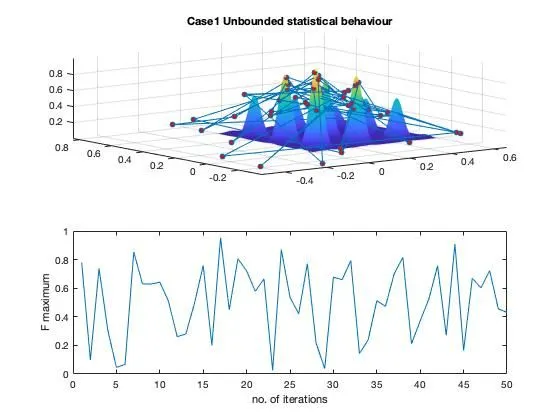
Figure 4: Graph Case1

• In 2nd case, in the first subplot we can see the peak points are only 4 which is better than the previous case. From the second subplot it seems the function values are changing between 0.7 to 1.

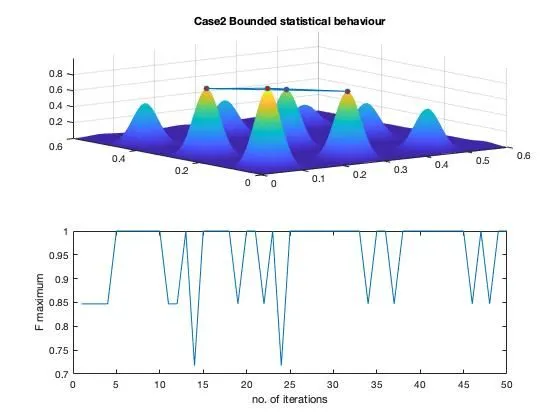
Figure 5: Graph Case2

• In 3rd case, in the first subplot only one peak point can be seen which is nothing but our maximum point. In the second subplot it can be seen that function values are changing for every iteration around same point which can be consider as 1, which is also the global maxima of the function. So by decreasing the search space for a higher populationsize ga will give similar results for every time it is run. The drawback in this case is that it takes time longer to execute than previous cases.

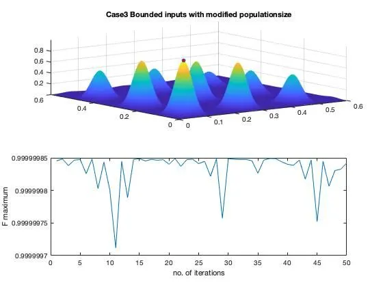
Figure 6: Graph Case3

• Below error is found while programming as variable f needs to follow loop counters f(i, j).

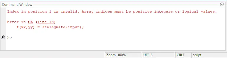
Figure 7: Error1

• Incorrect graph generated while programming because starting point is missing from the length/range of the for loop, therefore only the value at point 50 can be seen in the graph as range is missing. It is then corrected using range operator [for i = (1:iteration)].

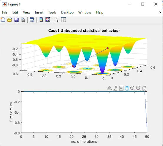
Figure 8: Error2

reference:-

• ga - https://in.mathworks.com/help/gads/ga.html#mw_a9a9e523-4242-481e-b6b9-acbe194a2432
• How the Genetic Algorithm Works - https://in.mathworks.com/help/gads/how-the-genetic-algorithm-works.html
• Find global minima for highly nonlinear problems - https://in.mathworks.com/discovery/genetic-algorithm.html?s_tid=srchtitle_genetic%20algorithm_2
• Genetic Algorithm Explained - https://skill-lync.com/knowledgebase/genetic-algorithm-explained