Week 3 - Solving second order ODEs

Solving second order ODEs

AIM:-

To write a program that solves the second order ODEs. This ODE represents the equation of motion of a simple pendulum with damping. Also to simulate angular displacement and angular velocity with respective time and to animate the motion of the pendulum.

Principle:-

Every second-order differential equation may be considered as a system of two first-order equations. This has a number of uses. In particular, it enables us to use first-order numerical methods to approximate the solution of a second-order initial value problem. In order to have a particular example, let's consider the second-order equation describing the motion of of a pendulum. A simple pendulum involves second order differential equation.

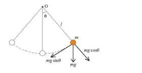
Solving for angle θ and rate at which θ value is changing with respective time which is velocity. In addition to this the same pendulum also describes the motion of a spring, mass and damper system. If the initial condition is given to the mass then the same ODE system can be use to describe how the mass is going to move. It has a lot of application in vehicle dynamics where suspension system can be modelled as a set of mass spring and dampers and can actually solve the ODE and figure out how vehicle dynamics is going to be. The fundamental idea behind ODE is both analytically and computational. When there is a higher order ODE then break it down into a set of first order ODE.

`(d^2theta)/dt^2` | 2nd ODE

`(d theta)/(dt)` | 1st ODE

In this case we have 2nd order ODE.

Let’s θ = θ1

`(d theta)/dt = (d theta1)/dt = theta2` | 1st relation

`(d^2theta)/dt^2 = d/dt*((d theta)/dt) = (d theta2)/dt` | 2nd relation

Original ODE -

`(d^2theta)/dt^2 + b/m*((d theta)/dt) + g/l*sintheta = 0`

By using 1st and 2nd relation-

`(d theta2)/dt + b/m*theta2 + g/l*sintheta1 =0`

To solve 2nd order ODE created two ODEs -

1 - `(d theta1)/dt =theta2`

2 - `(d theta2)/dt = -b/m*theta2 -g/l*sintheta1`

This is breaking down 2nd order ODE into a series of 1st order ODEs. The idea is about if we have 3rd order ODE then we can break it down into a system of three 1st order ODEs.

Lets say,

`d/dt*[[theta1],[theta2]] = [[theta2],[-b/m*theta1 -g/l*sintheta1]]`

lets call this L.H.S as θ. This is the solution vector because it’s contains two equations. When we try to save it using programming then it can be the ODE solvers in Matlab or Python. We need to provide the equation in this particular format.

Program:-

A function program is created and it is been merged into the main program to solve 2nd ODE. Below are the inputs taken for the program-

• damping coefficient(b) = 0.05
• gravity in m/s^2(g) = 9.81 m/s^2
• length of the pendulum in m(l) = 1 metre
• mass of the ball in kg(m) = 1 kg

• Solving for ODE system two 1st order ODE is needed 1st - displacement and 2nd - velocity. In 1st ODE we need to provide initial condition for displacement. Initial displacement of the pendulum is 0m and velocity is 3m/s. Integrating the ODE system to obtain a solution and for which we need to define the value for time. ’t_span’(time array) it goes from 0 to 20 sec for 500 values in between.

• Now we need to call a ODE function. ode45 is an inbuilt solver in Matlab and the original ODE which is ‘θ’ and ’t’ is the most important or main inputs. ’t’ and ‘θ’ are the dependent and independent variables of ODE system.

• Defining function ‘ode_func’ is ’t’ ,’θ’ followed by ‘b’, ‘g’, ‘l’, ‘m’ and after that we provide the initial condition ’t_span’ time array which is corresponding to the starting of the time. In funtion program the 1st ODE is dtheta1_dt = theta2 and 2nd ODE is dtheta2_dt = -(b/m)*theta2 - (g/l)*sintheta1. This function is going to give ’t’ time and ‘results’ and plot is made for the same.

function [dtheta_dt] = ode_func(t, theta, b, g, l, m)

theta1 = theta(1);
theta2 = theta(2);
dtheta1_dt = theta2;
dtheta2_dt = -(b/m)*theta2 - (g/l)*sin(theta1);
dtheta_dt = [dtheta1_dt; dtheta2_dt];

end

% 2nd ODE
clear all
close all
clc

% Inputs
b = 0.05;
g = 9.81;
l = 1;
m = 1;

% Initial condition
theta_0 = [0,3];

% Time points
t_span = linspace(0, 20, 500);

% ODE solve
[t, results] = ode45(@(t,theta) ode_func(t, theta, b, g, l, m), t_span, theta_0);

% Plot
plot(t, results(:,1))
hold on 
plot(t, results(:,2))
xlabel('time')
ylabel('plot')
legend ('angular displacement', 'angular velocity')
title('pendulum motion(displacement and velocity with respective time)')

% for loop
ct = 1;

for i = 1: length(t_span)

    x0 = 0;
    y0 = 0;
    x1 = l*sin(results(i,1));
    y1 = -l*cos(results(i,1));
    
% Pot1
figure(2)
plot([1 -1], [0 0], 'linewidth', 6, 'color', 'g')
hold on
plot([x0 x1], [y0 y1], 'linewidth', 3)
plot(x1, y1, 'O', 'MarkerSize', 20, 'MarkerFaceColor', 'y')
axis([-2 2 -2 2])
title('simulation of the pendulum motion')
hold off
M(ct) = getframe(gcf);
ct = ct + 1;
end

% Movie(animation)
movie(M)
videofile = VideoWriter('motion of a pendulum', 'MPEG-4');
open(videofile)
writeVideo(videofile, M)
close(videofile)

• A plot has been created of 't' and 'θ' by solving 2nd ODE with respective time. 'for loop' command is used with 'i' as a loop counter including coordinates (x0=0), (y0=0), (x1=l*sin(results(i,1))), (y1=-l*cos(results(i,1))) to simulate the motion of pendulum. By using 'marker' command sphere of a pendulum is also created.

• Finally an animation is made of the simulation using 'getframe(gcf)' command and taking counter as 'ct' and merging them together into 'movie(M)' command to create an animation.

Results:-

By solving 2nd ODE below plot is made which shows the motion of a pendulum with initial displacement as 0 and velocity as 3.

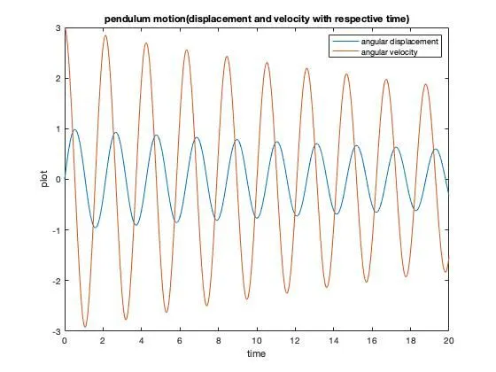
An animation is created of the simulation of motion of a simple pendulum.

Animation-

https://youtu.be/S9nyvvorbqw

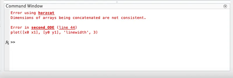
To resolve the above error x1 and y1 values was corrected. Colon was replaced by counter loop 'i' for results.

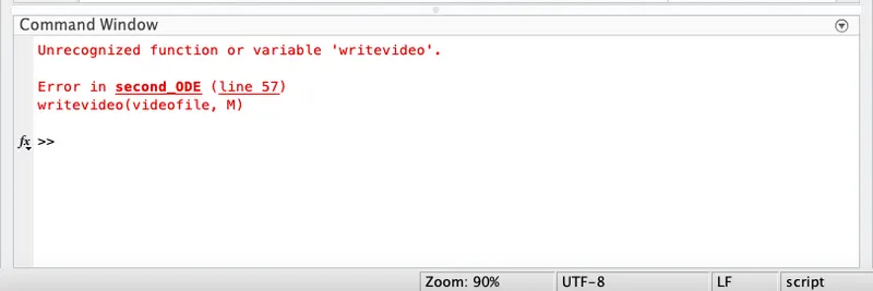
writevideo needs to be written in format writeVideo to get recognize by Matlab.