Project 2 - Rankine cycle Simulator
Rankine cycle Simulator
Aim:-
- Understand the concept of the Rankine cycle and create a Rankine cycle simulator using OCTAVE/MATLAB.
- Code should calculate the state points of the Rankine cycle and then, plot the corresponding T-s and h-s plots for the given set of inputs. Title and axes labels are a must, while legends could be used if necessary.
- Calculate Net work output and Back work ratio
Principle:-
The Rankine cycle is an idealized thermodynamic cycle describing the process by which certain heat engines, such as steam turbines or reciprocating steam engines, allow mechanical work to be extracted from a fluid as it moves between a heat source and heat sink. The Rankine cycle is named after William John Macquorn Rankine, a Scottish polymath professor at Glasgow University.
Heat energy is supplied to the system via a boiler where the working fluid (typically water) is converted to a high-pressure gaseous state (steam) to turn a turbine. After passing over the turbine, the fluid can condense back into a liquid state as waste heat energy is rejected before being returned to the boiler, completing the cycle. Friction losses throughout the system are often neglected to simplify calculations as such losses are usually much less significant than thermodynamic losses, especially in larger systems.
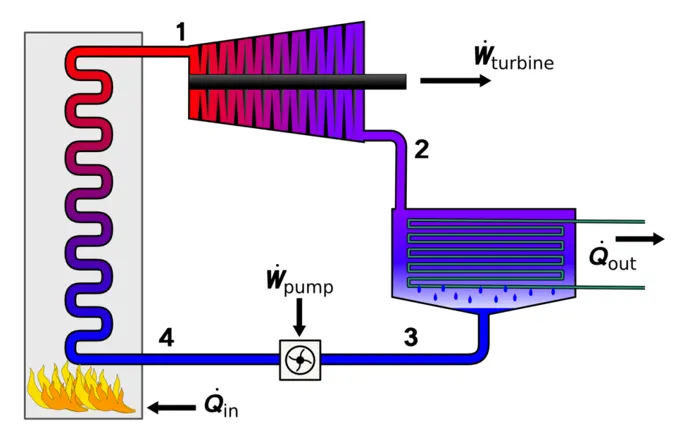
Figure 1. The physical layout of the Rankine Cycle
Description - The Rankine cycle closely describes the process by which steam engines commonly found in thermal power generation plants harness the thermal energy of a fuel or other heat source to generate electricity. Possible heat sources include the combustion of fossil fuels such as coal, natural gas, or oil, renewable fuels like biomass or ethanol, nuclear fission, and concentrated solar power. Common heat sinks include ambient air above or around a facility and bodies of water such as rivers, ponds, and oceans.
The ability of a Rankine engine to harness energy depends on the relative temperature difference between the heat source and heat sink. The greater the differential, the more mechanical power can be efficiently extracted out of heat energy, as per Carnot's theorem.
Rankine engines generally operate in a closed-loop where the working fluid is reused. The water vapor with condensed droplets often seen billowing from power stations is created by the cooling systems (not directly from the closed-loop Rankine power cycle). This 'exhaust' heat is represented by the "Qout" flowing out of the lower side of the cycle shown in the T–s diagram below. Cooling towers operate as large heat exchangers by absorbing the latent heat of vaporization of the working fluid and simultaneously evaporating cooling water into the atmosphere.
While many substances can be used as the working fluid, water is usually chosen for its simple chemistry, relative abundance, low cost, and thermodynamic properties. By condensing the working steam vapor to a liquid the pressure at the turbine outlet is lowered and the energy required by the feed pump consumes only 1% to 3% of the turbine output power these factors contribute to higher efficiency for the cycle. This benefit is offset by the low temperatures of steam admitted to the turbine(s). Gas turbines, for instance, have turbine entry temperatures approaching 1500 °C. However, the thermal efficiency of large steam power stations and large modern gas turbine stations is similar.
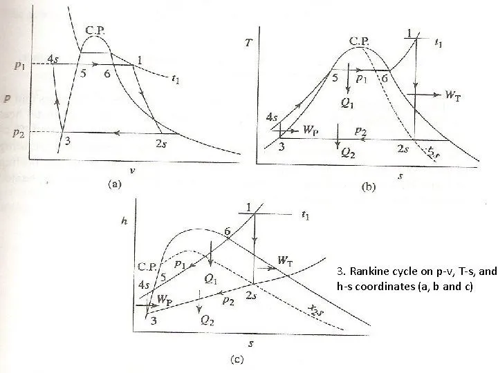
Figure 2. p-v, T-s, and h-s diagram of Rankine Cycle
Processes in the Rankine cycle - There are four processes in the Rankine cycle.
- Process 1–2: The dry saturated vapor expands through a turbine, generating power. This decreases the temperature and pressure of the vapor, and some condensation may occur. The output in this process can be easily calculated using the chart or tables noted above. Process 1-2 is isentropic expansion.
- Process 2–3: The wet vapor then enters a condenser, where it is condensed at a constant pressure to become a saturated liquid. Process 2-3 is constant pressure heat rejection in the condenser.
- Process 3–4: The working fluid is pumped from low to high pressure. As the fluid is a liquid at this stage, the pump requires little input energy. Process 3-4 is isentropic compression.
- Process 4–1: The high-pressure liquid enters a boiler, where it is heated at constant pressure by an external heat source to become a dry saturated vapor. The input energy required can be easily calculated graphically, using an enthalpy–entropy chart (h–s chart), or numerically, using steam tables or software. Process 4-1 is constant pressure heat addition in the boiler.
In an ideal Rankine cycle, the pump and turbine would be isentropic, i.e., the pump and turbine would generate no entropy and hence maximize the network output. Processes 1–2 and 3–4 would be represented by vertical lines on the T–s diagram and more closely resemble that of the Carnot cycle. The Rankine cycle shown here prevents the state of the working fluid from ending up in the superheated vapor region after the expansion in the turbine, [1] which reduces the energy removed by the condensers.
Equation -
- h2 = hf2+(x2*(hg2-hf2)) | x2 = (s2-sf2)/(sg2-sf2) | hf2 = XSteam(‘hL_p’, p2) | hg2 = XSteam(‘hV_p’, p2) | sf2 = XSteam(’sL_p’, p2) | sg2 = XSteam(‘sV_p’, p2)
- T4 = T3*((p4/p3)^(gamma-1)/gamma) | gamma = Cp1/Cv1 | Cp1 = XSteam(‘CpL_p’, p4) | Cv1 = XSteam(‘CvL_p’, p4)
- h4 = Wp+h3 | Wp = v3*(p4/p3)*100
- Wt = h1-h2
- Wnet = Wt+Wp
- Bwr = (h4-h3)/(h1-h2)
Where,
T = Temperature (deg C) | p = Pressure (bar) | h = Enthalpy (KJ/kg) | s = Entropy (KJ/K) | v = Volume (m3/kg) | Wt = Work done by Turbine | Wp = Work done to run Pump | Wnet = Net work done | Bwr = Back work ratio | Cp = Specific isobaric heat capacity | Cv = Specific isochoric heat capacity | f determines liquid state and g determines vapour/gas state of water.
- Enthalpy is a thermodynamic property of a system. It is the sum of the internal energy added to the product of the pressure and volume of the system. It reflects the capacity to do non-mechanical work and the capacity to release heat. Enthalpy is denoted as H; specific enthalpy is denoted as h.
- The entropy of an object is a measure of the amount of energy that is unavailable to do work. Entropy is also a measure of the number of possible arrangements the atoms in a system can have. In this sense, entropy is a measure of uncertainty or randomness. Specific enthalpy is denoted as s.
Program:-
Standard Xsteam library is used to get the steam table data for water. It is used to calculate the points in between the state variables.
% Rankine Cycle Simulator
% [1-2] Isentropic expansion in the turbine
% [2-3] Constant pressure heat rejection by the condenser
% [3-4] Isentropic compression in the pump
% [4-1] Constant pressure heat addition by the boiler
clear all
close all
clc

% Inputs
% T Temperature (deg C)
T1 = 400;
% p Pressure (bar)
p1 = 30;
p2 = 0.05;


% State point 1
% Enthalpy at state point 1
% h_pT Entalpy as a function of pressure and temperature.
h1 = XSteam('h_pT', p1, T1 );
% Entropy at state point 1
% s_pT Specific entropy as a function of pressure and temperature (Returns saturated vapour entalpy if mixture.)
s1 = XSteam('s_pT', p1, T1);

% State point 2 | [1-2] isentropic expansion
% Entropy at state point 2
s2 = s1;
% Temperature at state point 2
% Tsat_p Saturation temperature
T2 = XSteam('Tsat_p', p2);
% Enthalpy at state point 2
% sL_p Saturated liquid entropy
sf2 = XSteam('sL_p', p2);
% sV_p Saturated vapour entropy
sg2 = XSteam('sV_p', p2);
% hL_p Saturated liquid enthalpy
hf2 = XSteam('hL_p', p2);
% hV_p Saturated vapour enthalpy
hg2 = XSteam('hV_p', p2);
x2 = (s2-sf2)/(sg2-sf2);
h2 = hf2+(x2*(hg2-hf2));

% State point 3 | [2-3] constant pressure heat rejection
p3 = p2;
% Volume at state point 3
% vL_p Saturated liquid volume
v3 = XSteam('vL_p', p3);
% Temperature at state point 3 | Tsat_p Saturation temperature
T3 = T2;
% Enthalpy at state point 3
% hL_T Saturated liquid enthalpy
h3 = XSteam('hL_T', T3 );
% Entropy at state point 3
% sL_T Saturated liquid entropy
s3 = XSteam('sL_T', T3);

% State point 4 | [3-4] isentropic compression | [4-1] constant pressure heat addition
p4 = p1;
% Entropy at state point 4
s4 = s3;
% Specific isobaric heat capacity(Cp)
% Cp_ps Specific isobaric heat capacity as a function of pressure and entropy.
Cp1 = XSteam('Cp_ps', p4, s4);
% Specific isochoric heat capacity(Cp)
% Cv_ps Specific isochoric heat capacity as a function of pressure and entropy.
Cv1 = XSteam('Cv_ps', p4, s4);
gamma = Cp1/Cv1;
% Temperature at state point 4
T4 = T3*((p4/p3)^(gamma-1/gamma));
% Enthalpy at state point 4
% Work done to run pump
Wp = v3*(p4-p3)*100;
h4 = Wp + h3;

% Saturation process(Saturated liquid - Saturated vapour) during [4-1]
% Tsat_p Saturation temperature
T5 = XSteam('Tsat_p', p4);
% hL_p Saturated liquid enthalpy
h5 = XSteam('hL_p', p4);
% sL_p Saturated liquid entropy
s5 = XSteam('sL_p', p4);
% According to T-s graph
T6 = T5;
% hV_p Saturated vapour enthalpy
h6 = XSteam('hV_p', p1);
% sV_p Saturated vapour entropy
s6 = XSteam('sV_p', p1);

% To create saturation curve for T-s and h-s diagram
% Temperature array
T = linspace(0, 400, 500);
for i = 1:length(T)
    % hL_T Saturated liquid enthalpy
    hf(i) = XSteam('hL_T', T(i));
    % sL_T Saturated liquid entropy
    sf(i) = XSteam('sL_T', T(i));
    % hV_T Saturated vapour enthalpy
    hg(i) = XSteam('hV_T', T(i));
    % sV_T Saturated vapour entropy
    sg(i) = XSteam('sV_T', T(i));
end

% Net work
% Work done by turbine
Wt = h1-h2;
Wnet = Wt-Wp;

% Back work ratio
Bwr = (h4-h3)/(h1-h2);

% Plot
% Temperature vs entropy
hold on
plot([sf sg], [T T], 'r', 'linewidth', 2)
text(s1, T1, '1', 'fontsize', 15)
plot([s1 s2], [T1 T2], 'black', 'linewidth', 2)
text(s2, T2, '2', 'fontsize', 15)
plot([s2 s3], [T2 T3], 'black', 'linewidth', 2)
text(s3, T3, '3', 'fontsize', 15)
plot([s3 s4], [T3 T4], 'black', 'linewidth', 2)
text(s4, T4, '4', 'fontsize', 15)
plot([s4 s5], [T4 T5], 'black', 'linewidth', 2)
plot([s5 s6], [T5 T6], 'black', 'linewidth', 2)
plot([s6 s1], [T6 T1], 'black', 'linewidth', 2)
title('temperature vs entroy', '(T) vs (s)')
xlabel('entropy(s)')
ylabel('Temperature(T)')
legend('Saturation curve', 'location', 'northwest')

% enthalpy vs entropy
figure(2)
hold on
plot([sf sg], [hf hg], 'r', 'linewidth', 2)
text(s1, h1, '1', 'fontsize', 15)
plot([s1 s2], [h1 h2], 'black', 'linewidth', 2)
text(s2, h2, '2', 'fontsize', 15)
plot([s2 s3], [h2 h3], 'black', 'linewidth', 2)
text(s3, h3, '3', 'fontsize', 15)
plot([s3 s4], [h3 h4], 'black', 'linewidth', 2)
text(s4, h4, '4', 'fontsize', 15)
plot([s4 s1], [h4 h1], 'black', 'linewidth', 2)
title('enthalpy vs entroy', '(h) vs (s)')
xlabel('entropy(s)')
ylabel('enthalpy(h)')
legend('Saturation curve', 'location', 'northwest')- Based on the 4 processes of the Rankine cycle all the state variables of the cycle can be determine. With the help of the given inputs and using the XSteam function enthalpy and entropy if state point 1 is determined. This state point follows process [1-2] i.e isentropic expansion and [4-1] i.e constant pressure heat addition by the boiler. Similarly, every state point follows two corresponding processes, which can be used to determine the state variables of that state point.
- At state point 2 due to the process [1-2] i.e isentropic expansion, entropy at state point 2 will be constant. The temperature at state point 2 is found using XSteam function saturation temperature. Using the equation for h2, the enthalpy of this point is calculated.
- At state point 3, process [2-3] will apply i.e constant pressure heat rejection where the pressure at state point 3 will be constant and considering the same volume is determined. The temperature will be equal to the temperature of state point 2 as both use XSteam function saturation temperature. Enthalpy and entropy are calculated using the XSteam function saturated liquid enthalpy and saturated liquid entropy.
- At state point 4, process [4-1] is applied i.e constant pressure heat addition, therefore pressure will be constant. Process [3-4] also applies to state point 4 i.e isentropic compression hence entropy will be constant. By the equation of T4 and h4 temperature and enthalpy are being calculated.
- For every process phases of the water i.e liquid and vapor/gas are also considered. At state points 4 and 1 saturation process takes place where water is boiled and converted into a saturated liquid state and then it is converted to the saturated vapor state and then due to more boiling inside the boiler is converted to a superheated state. Two different phases are taking place between state points 4 and 1 hence temperature, enthalpy, and entropy for both the phases are calculated.
- To create a saturation curve for T-s and h-s diagram different enthalpy and entropy values based on liquid state and vapor/gas state are being calculated using temperature as an array for values 0 to 400 considering 500 values in between them. Net work done is calculated by equating work done by the turbine and work done to run the pump, using the equation of Wnet. The back work ratio is calculated using the equation for Bwr.
- Plots are created for T-s and h-s using the ‘hold on’ command for all the state points. At first saturation, the curve is made for both the graphs using h and s values that were calculated with temperature array at different phases of water. Then all the state points are joined using the ‘plot’ command. The t-s and h-s diagram includes title, axis labels and legends, and ‘text’ command to show the state points of the graph.
Results:-
Below are the T-s and h-s diagrams generated through the program based on the given inputs. Both diagrams represent the Rankine cycle and how temperature and enthalpy change in the complete cycle.
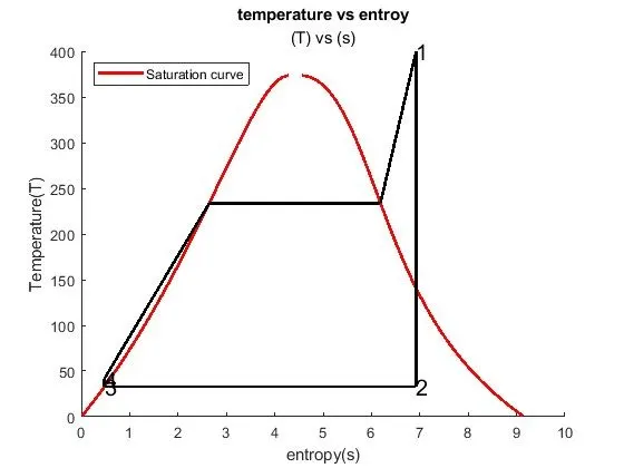
Figure 3. T-s diagram generated through the program
- In the T-s diagram, it can be seen how temperature changes throughout the process of the cycle. In the saturation curve, the left side is the saturated liquid state line and the right side is the saturated vapor/gas state line. In between state points [4-1] water changes from saturated liquid to saturated vapor/gas and then it goes to a superheated state. This is how high-pressure steam is formed.
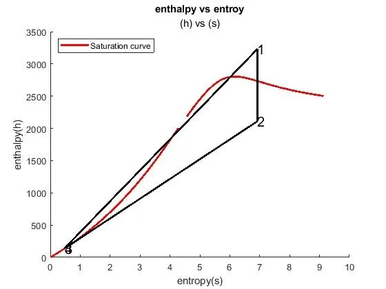
Figure 4. h-s diagram generated through the program
- In the h-s diagram, it can be seen how enthalpy changes during the cycle. The first part of the saturation curve is the saturated liquid state and the second part is the saturated vapor/gas state. Enthalpy increases with an increase in heat energy.
Output -
Below are the values of all the state variables, the Net work done, the Back work ratio, and all rest of the variables to calculate the same.
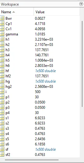
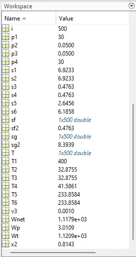
Figure 5. Results of the entire program
Error:-
Error (I) was resolved by giving single quotes to the input of the function.

Figure 6. Error (I)
Error (II) was resolved by altering the positions of the state points of entropy.

Figure 7. Error (II)
Reference:-
Rankine Cycle - https://en.wikipedia.org/wiki/Rankine_cycle