Week 3.5 - Deriving 4th order approximation of a 2nd order derivative using Taylor Table method
Deriving 4th order approximation of a 2nd order derivative using Taylor Table method
Derive the following 4th-order approximations of the second-order derivative as :
1. Central difference
2. Skewed right-sided difference
3. Skewed left-sided difference
1. Central difference 4th-order approximation of the 2nd order derivative:
For deriving the central difference of a 4th order approximation/accuracy of a 2nd order derivative, firstly we have to determine the no. of nodes known as the numerical stencil. So let's go
number of nodes`n= (p+q)-1`
here, n=no. of nodes
p=order of derivative, which is '2' for this problem
q=order of the approximation which is of the '4th order' for this problem
so,
number of nodes`n=(2+4)-1=5`
so here, we have '5' nodes in a central difference on which we are going to make a discretization i.e., to find the value of an arbitrary function for the 2nd order derivative & that '5' nodes in a central difference are as:
(i-2) (i-1) i (i+1) (i+2)
In central difference, we go from the center as you can see in the above nodes that we go 2 units from 'i' to the left as '(i-1)' & '(i-2)' as well as to the right as '(i+1)' & '(i+2)'.
So, now I think that after such a basic explanation, I can go for deriving the numerical scheme as of central difference using the Taylor table method as:
(i) Hypothetical equation:
`(di^2)*d^2/dx^2(f(i))=a*f(i-2)+b*f(i-1)+c*f(i)+d*f(i+1)+e*f(i+2)`
(ii) Expanding each of the above equation terms on R.H.S. (for Taylor table) using the Taylor series expansion method:
`a*f(i-2)=a*f(i)-a*f'(i)*(2*di)+a*f''(i)*(2*di)^2/(2!)-a*f'''(i)*(2*di)^3/(3!)+a*f''''(i)*(2*di)^4/(4!)`
`b*f(i-1)=b*f(i)-b*f'(i)*(di)+b*f''(i)*(di)^2/(2!)-b*f'''(i)*(di)^3/(3!)+b*f''''(i)*(di)^4/(4!)`
`c*f(i)=c*f(i)`
`d*f(i+1)=d*f(i)+d*f'(i)*(di)+d*f''(i)*(di)^2/(2!)+d*f'''(i)*(di)^3/(3!)+d*f''''(i)*(di)^4/(4!)`
`e*f(i+2)=e*f(i)+e*f'(i)*(2*di)+e*f''(i)*(2*di)^2/(2!)+e*f'''(i)*(2*di)^3/(3!)+e*f''''(i)*(2*di)^4/(4!)`
(iii). Using the above equations in '(ii)' in the Taylor table as follows:
| `(di^2)*d^2/dx^2(f(i))` | `f(i)` | `f'(i)*di` | `f''(i)*(di^2)/(2!)` | `f'''(i)*(di^3)/(3!)` | `f''''(i)*(di^4)/(4!)` | |
| `a*f(i-2)` | `a` | `-2*a` | `4*a` | `-8*a` | `16*a` | |
| `b*f(i-1)` | `b` | `-b` | `b` | `-b` | `b` | |
| `c*f(i)` | `c` | `0` | `0` | `0` | `0` | |
| `d*f(i+1)` | `d` | `d` | `d` | `d` | `d` | |
| `e*f(i+2)` | `e` | `2*e` | `4*e` | `8*e` | `16*e` | |
| `sum=(di^2)*d^2/dx^2(f(i))` | `0` | `0` | `1` | `0` | `0` |
(iv). Writing the coefficients of the column header of the above table into the equation form as follows:
`d^2/dx^2(f(i))=(a*f(i-2)+b*f(i-1)+c*f(i)+d*f(i+1)+e*f(i+2))/(di^2)=`
`a+b+c+d+e=0`
`(-2*a)-b+0+d+(2*e)=0`
`(4*a)/2+b/2+0+d/2+(4*e)/2=1`
`(-8*a)/6-b/6+0+d/6+(8*e)/6=0`
`(16*a)/24+b/24+0+d/24+(16*e)/24=0`
As we have got the above system of equations from the Taylor table method. So we need to solve these systems of equations which we will be going to solve (to derive the required numerical scheme) in a MATLAB by programming as:
% solving the system of equations of the central difference of 4th order
% approximation for the 2nd order derivative as


% system of equations

% a+b+c+d+e=0
% (-2*a)-b+0+d+(2*e)=0
% (4*a)/2+b/2+0+d/2+(4*e)/2=1
% (-8*a)/6-b/6+0+d/6+(8*e)/6=0
% (16*a)/24+b/24+0+d/24+(16*e)/24=0


clear all
close all
clc

% coefficients of the variables 'a', 'b', 'c', 'd' & 'e' of the system of
% equations
A=[1 1 1 1 1;-2 -1 0 1 2;4/2 1/2 0 1/2 4/2;-8/6 -1/6 0 1/6 8/6;16/24 1/24 0 1/24 16/24]

% R.H.S. of the system of equations
B=[0;0;1;0;0]


% solving the system of equations from the matrice format of 'AX=B'
format rational       % To get the values in fractional terms
x=A^-1*B              % AX=B, but for X, it is X=A^-1*B
The output is a solved system of equations by solving for the variables 'a', 'b', 'c', 'd' & 'e' by MATLAB as follows in the screenshot of the command window:
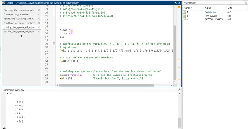
So as you can see above that we got the '5' values of x which are nothing but just the value of 'a'=-1/12, 'b'=4/3, 'c'=-5/2, 'd'=4/3, 'e'=-1/12
We are going to substitute these values in the above (i) hypothetical equation of the Taylor table method as:
`d^2/dx^2(f(i))=(-1/12*f(i-2)+4/3*f(i-1)-5/2*f(i)+4/3*f(i+1)-1/12*f(i+2))/(di^2)`
The above derived numerical scheme is the central difference 4th order accuracy of the 2nd order derivative.
Proof for 4th order accuracy of the above derived numerical scheme as:
The order of accuracy (P) = Number of nodes in the stencil (N) - order of derivative (Q) + 1 for symmetric/central schemes so
`P=(N-Q)+1=(5-2)+1=4`
2. Skewed right-sided difference:
Skewed right-sided difference 4th-order approximation of the 2nd order derivative:
For deriving the Skewed right-sided difference of a 4th order approximation/accuracy of a 2nd order derivative, firstly we have to determine the no. of nodes in a numerical stencil for a skewed right-sided difference of a 4th order approximation/accuracy of a 2nd order derivative. So let's go
number of nodes`n= p+q`
here, n=no. of nodes
p=order of derivative, which is '2' for this problem
q=order of the approximation which is of the '4th order' for this problem
so,
number of nodes`n=2+4=6`
so here, we have '6' nodes in a skewed right-sided difference on which we are going to make a discretization i.e., to find the value of an arbitrary function for the 2nd order derivative & that '6' nodes in a skewed right-sided difference are as:
i (i+1) (i+2) (i+3) (i+4) (i+5)
In skewed right-sided difference, we go to the right as you can see in the above nodes that we go one by one units from 'i' to the right as '(i+1)', '(i+2)', '(i+3)', '(i+4)' & '(i+5)', that's why the positive(+) sign is here.
So, now I think that after such a basic explanation, I can go for deriving the numerical scheme as of the skewed right-sided difference using the Taylor table method as:
(i). Hypothetical equation:
`(di^2)*d^2/dx^2(f(i))=a*f(i)+b*f(i+1)+c*f(i+2)+d*f(i+3)+e*f(i+4)+g*f(i+5)`
(ii) Expanding each of the above equation terms on R.H.S. (for Taylor table) using the Taylor series expansion method:
`a*f(i)=a*f(i)`
`b*f(i+1)=b*f(i)+b*f'(i)*(di)+b*f''(i)*(di^2)/(2!)+b*f'''(i)*(di^3)/(3!)+b*f''''(i)*(di^4)/(4!)+b*f'''''(i)*(di^5)/(5!)`
`c*f(i+2)=c*f(i)+c*f'(i)*(2*di)+c*f''(i)*(2*di)^2/(2!)+c*f'''(i)*(2*di)^3/(3!)+c*f''''(i)*(2*di)^4/(4!)+c*f'''''(i)*(2*di)^5/(5!)`
`d*f(i+3)=d*f(i)+d*f'(i)*(3*di)+d*f''(i)*(3*di)^2/(2!)+d*f'''(i)*(3*di)^3/(3!)+d*f''''(i)*(3*di)^4/(4!)+d*f'''''(i)*(3*di)^5/(5!)`
`e*f(i+4)=e*f(i)+e*f'(i)*(4*di)+e*f''(i)*(4*di)^2/(2!)+e*f'''(i)*(4*di)^3/(3!)+e*f''''(i)*(4*di)^4/(4!)+e*f'''''(i)*(4*di)^5/(5!)`
`g*f(i+5)=g*f(i)+g*f'(i)*(5*di)+g*f''(i)*(5*di)^2/(2!)+g*f'''(i)*(5*di)^3/(3!)+g*f''''(i)*(5*di)^4/(4!)+g*f'''''(i)*(5*di)^5/(5!)`
(iii). Using the above equations in '(ii)' in the Taylor table as follows:
| `(di^2)*d^2/dx^2(f(i))` | `f(i)` | `f'(i)*di` | `f''(i)*(di^2)/(2!)` | `f'''(i)*(di^3)/(3!)` | `f''''(i)*(di^4)/(4!)` | `f'''''(i)*(di^5)/(5!)` |
| `a*f(i)` | `a` | `0` | `0` | `0` | `0` | `0` |
| `b*f(i+1)` | `b` | `b` | `b` | `b` | `b` | `b` |
| `c*f(i+2)` | `c` | `2*c` | `4*c` | `8*c` | `16*c` | `32*c` |
| `d*f(i+3)` | `d` | `3*d` | `9*d` | `27*d` | `81*d` | `243*d` |
| `e*f(i+4)` | `e` | `4*e` | `16*e` | `64*e` | `256*e` | `1024*e` |
| `g*f(i+5)` | `g` | `5*g` | `25*g` | `125*g` | `625*g` | `3125*g` |
| `sum=(di^2)*d^2/dx^2(f(i))` | `0` | `0` | `1` | `0` | `0` | 0 |
(iv). Writing the coefficients of the column header of the above table into the equation form as follows:
`d^2/dx^2(f(i))=(a*f(i)+b*f(i+1)+c*f(i+2)+d*f(i+3)+e*f(i+4)+g*f(i+5))/(di^2)=`
`a+b+c+d+e+g=0`
`0+b+(2*c)+(3*d)+(4*e)+(5*g)=0`
`0+b/2+(4*c)/2+(9*d)/2+(16*e)/2+(25*g)/2=1`
`0+b/6+(8*c)/6+(27*d)/6+(64*e)/6+(125*g)/6=0`
`0+b/24+(16*c)/24+(81*d)/24+(256*e)/24+(625*g)/24=0`
`0+b/120+(32*c)/120+(243*d)/120+(1024*e)/120+(3125*g)/120=0`
As we have got the above system of equations from the Taylor table method. So we need to solve these systems of equations which we will be going to solve (to derive the required numerical scheme) in a MATLAB by programming as:
% solving the system of equations of the skewed right-sided difference of
% 4th order approximation for the 2nd order derivative


% system of equations
% a+b+c+d+e+g=0
% 0+b+(2*c)+(3*d)+(4*e)+(5*g)=0
% 0+b/2+(4*c)/2+(9*d)/2+(16*e)/2+(25*g)/2=1
% 0+b/6+(8*c)/6+(27*d)/6+(64*e)/6+(125*g)/6=0
% 0+b/24+(16*c)/24+(81*d)/24+(256*e)/24+(625*g)/24=0
% 0+b/120+(32*c)/120+(243*d)/120+(1024*e)/120+(3125*g)/120=0


clear all
close all
clc


% coefficients of the variables 'a', 'b', 'c', 'd', 'e' & 'g' of the system of
% equations
A=[1 1 1 1 1 1;0 1 2 3 4 5;0 1/2 4/2 9/2 16/2 25/2;0 1/6 8/6 27/6 64/6 125/6;0 1/24 16/24 81/24 256/24 625/24;0 1/120 32/120 243/120 1024/120 3125/120]

% R.H.S. of the system of equations
B=[0;0;1;0;0;0]


% solving the system of equations from the matrice format of 'AX=B'
format rational          % To get the values in fractional terms
X=A^-1*B                 % AX=B, but for X, it is X=A^-1*B
The output is a solved system of equations by solving for the variables 'a', 'b', 'c', 'd', 'e' & 'g' by MATLAB as follows in the screenshot of the command window:
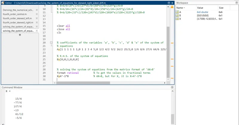
So as you can see above that we got the '6' values of x which are nothing but just the value of 'a'=15/4, 'b'=-77/6, 'c'=107/6, 'd'=-13, 'e'=61/12 & 'g'=-5/6
We are going to substitute these values in the above (i) hypothetical equation of the Taylor table method as:
`d^2/dx^2(f(i))=((15/4)*f(i)-(77/6)*f(i+1)+(107/6)*f(i+2)-13*f(i+3)+(61/12)*f(i+4)-(5/6)*f(i+5))/(di^2)`
The above derived numerical scheme is the skewed right-sided difference 4th order accuracy of the 2nd order derivative.
Proof for 4th order accuracy of the above derived numerical scheme as:
The order of accuracy P = Number of nodes in the stencil N - order of derivative Q for one-sided/skewed schemes
`P=(N-Q)=(6-2)=4`
3. Skewed left-sided difference:
Skewed left-sided difference 4th-order approximation of the 2nd order derivative:
For deriving the Skewed left-sided difference of a 4th order approximation/accuracy of a 2nd order derivative, firstly we have to determine the no. of nodes in a numerical stencil for a skewed left-sided difference of a 4th order approximation/accuracy of a 2nd order derivative. So let's go
number of nodes`n= p+q`
here, n=no. of nodes
p=order of derivative, which is '2' for this problem
q=order of the approximation which is of the '4th order' for this problem
so,
number of nodes`n=2+4=6`
so here, we have '6' nodes in a skewed left-sided difference on which we are going to make a discretization i.e., to find the value of an arbitrary function for the 2nd order derivative & that '6' nodes in a skewed left-sided difference are as:
(i-5) (i-4) (i-3) (i-2) (i-1) (i)
In skewed left-sided difference, we go to the left as you can see in the above nodes that we go one by one unit from 'i' to the left as '(i-1)', '(i-2)', '(i-3)', '(i-4)' & '(i-5)', that's why the negative(-) sign is here.
So, now I think that after such a basic explanation, I can go for deriving the numerical scheme as of the skewed left-sided difference using the Taylor table method as:
(i). Hypothetical equation:
`(di^2)*d^2/dx^2(f(i))=a*f(i-5)+b*f(i-4)+c*f(i-3)+d*f(i-2)+e*f(i-1)+g*f(i)`
(ii) Expanding each of the above equation terms on R.H.S. (for Taylor table) using the Taylor series expansion method:
`a*f(i-5)=a*f(i)-a*f'(i)*(5*di)+a*f''(i)*(5*di)^2/(2!)-a*f'''(i)*(5*di)^3/(3!)+a*f''''(i)*(5*di)^4/(4!)-a*f'''''(i)*(5*di)^5/(5!)`
`b*f(i-4)=b*f(i)-b*f'(i)*(4*di)+b*f''(i)*(4*di)^2/(2!)-b*f'''(i)*(4*di)^3/(3!)+b*f''''(i)*(4*di)^4/(4!)-b*f'''''(i)*(4*di)^5/(5!)`
`c*f(i-3)=c*f(i)-c*f'(i)*(3*di)+c*f''(i)*(3*di)^2/(2!)-c*f'''(i)*(3*di)^3/(3!)+c*f''''(i)*(3*di)^4/(4!)-c*f'''''(i)*(3*di)^5/(5!)`
`d*f(i-2)=d*f(i)-d*f'(i)*(2*di)+d*f''(i)*(2*di)^2/(2!)-d*f'''(i)*(2*di)^3/(3!)+d*f''''(i)*(2*di)^4/(4!)-d*f'''''(i)*(2*di)^5/(5!)`
`e*f(i-1)=e*f(i)-e*f'(i)*(di)+e*f''(i)*(di^2)/(2!)-e*f'''(i)*(di^3)/(3!)+e*f''''(i)*(di^4)/(4!)-e*f'''''(i)*(di^5)/(5!)`
`a*f(i)=a*f(i)`
(iii). Using the above equations in '(ii)' in the Taylor table as follows:
| `(di^2)*d^2/dx^2(f(i))` | `f(i)` | `f'(i)*di` | `f''(i)*(di^2)/(2!)` | `f'''(i)*(di^3)/(3!)` | `f''''(i)*(di^4)/(4!)` | `f'''''(i)*(di^5)/(5!)` |
| `a*f(i-5)` | `a` | `-5*a` | `25*a` | `-125*a` | `625*a` | `-3125*a` |
| `b*f(i-4)` | `b` | `-4*b` | `16*b` | `-64*b` | `256*b` | `-1024*b` |
| `c*f(i-3)` | `c` | `-3*c` | `9*c` | `-27*c` | `81*c` | `-243*c` |
| `d*f(i-2)` | `d` | `-2*d` | `4*d` | `-8*d` | `16*d` | `-32*d` |
| `e*f(i-1)` | `e` | `-e` | `e` | `-e` | `e` | `-e` |
| `g*f(i)` | `g` | 0 | `0` | `0` | `0` | `0` |
| `sum=(di^2)*d^2/dx^2(f(i))` | `0` | `0` | `1` | `0` | `0` | `0` |
(iv). Writing the coefficients of the column header of the above table into the equation form as follows:
`d^2/dx^2(f(i))=(a*f(i-5)+b*f(i-4)+c*f(i-3)+d*f(i-2)+e*f(i-1)+g*f(i))/(di^2)=`
`a+b+c+d+e+g=0`
`(-5*a)-(4*b)-(3*c)-(2*d)-e+0=0`
`(25/2)*a+(16/2)*b+(9/2)*c+(4/2)*d+e/2+0=1`
`(-125/6)*a-(64/6)*b-(27/6)*c-(8/6)*d-(e/6)=0`
`(625/24)*a+(256/24)*b+(81/24)*c+(16/24)*d+(e/24)=0`
`(-3125/120)*a-(1024/120)*b-(243/120)*c-(32/120)*d-e/120=0`
As we have got the above system of equations from the Taylor table method. So we need to solve these systems of equations which we will be going to solve (to derive the required numerical scheme) in a MATLAB by programming as:
% solving the system of equations of the skewed left-sided difference of
% 4th order approximation for the 2nd order derivative


% system of equations

% a+b+c+d+e+g=0
% (-5*a)-(4*b)-(3*c)-(2*d)-e+0=0
% (25/2)*a+(16/2)*b+(9/2)*c+(4/2)*d+e/2+0=1
% (-125/6)*a-(64/6)*b-(27/6)*c-(8/6)*d-(e/6)=0
% (625/24)*a+(256/24)*b+(81/24)*c+(16/24)*d+(e/24)=0
% (-3125/120)*a-(1024/120)*b-(243/120)*c-(32/120)*d-e/120=0


clear all
close all
clc


% coefficients of the variables 'a', 'b', 'c', 'd', 'e' & 'g' of the system
% of equations
A=[1 1 1 1 1 1;-5 -4 -3 -2 -1 0;25/2 16/2 9/2 4/2 1/2 0;-125/6 -64/6 -27/6 -8/6 -1/6 0;625/24 256/24 81/24 16/24 1/24 0;-3125/120 -1024/120 -243/120 -32/120 -1/120 0]


% R.H.S. of the system of equations
B=[0;0;1;0;0;0]


% solving the system of equations from the matrice format of 'AX=B'
format rational         % To get the values in fractional terms
X=A^-1*B                % AX=B, but for X, it is X=A^-1*B
The output is a solved system of equations by solving for the variables 'a', 'b', 'c', 'd', 'e' & 'g' by MATLAB as follows in the screenshot of the command window:
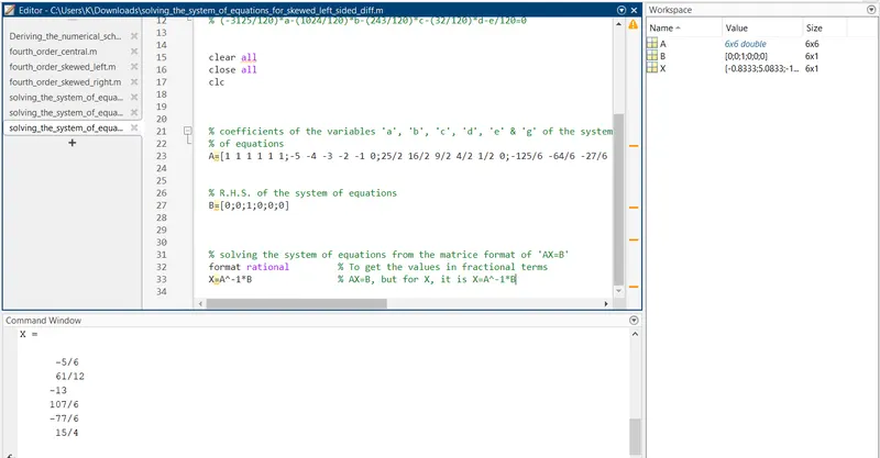
So as you can see above that we got the '6' values of x which are nothing but just the value of 'a'=-5/6, 'b'=61/12, 'c'=-13, 'd'=107/6, 'e'=-77/6 & 'g'=15/4
We are going to substitute these values in the above (i) hypothetical equation of the Taylor table method as:
`d^2/dx^2(f(i))=((-5/6)*f(i-5)+(61/12)*f(i-4)-13*f(i-3)+(107/6)*f(i-2)-(77/6)*f(i-1)+(15/4)*f(i))/(di^2)`
The above derived numerical scheme is the skewed left-sided difference 4th order accuracy of the 2nd order derivative.
Proof for 4th order accuracy of the above derived numerical scheme as:
The order of accuracy P = Number of nodes in the stencil N - order of derivative Q for one-sided/skewed schemes
`P=(N-Q)=(6-2)=4`
After deriving the above-asked numerical schemes, I make a function of these numerical schemes in MATLAB so that I can use these functions again & again to evaluate the second-order derivative of the given analytical function exp(x)*cos(x). The MATLAB functions are as follows:
Now, I am explaining each function one by one as
1. function for the fourth order approx using the central difference
% function for the fourth order approx using the central difference

function[fourth_order_error_c]=fourth_order_central(x,dx)

analytical_derivative=-2*exp(x)*sin(x)

fourth_order_approx=((-1/12)*(exp(x-2*dx)*cos(x-2*dx))+(4/3)*(exp(x-dx)*cos(x-dx))-(5/2)*(exp(x)*cos(x))+(4/3)*(exp(x+dx)*cos(x+dx))-(1/12)*(exp(x+2*dx)*cos(x+2*dx)))/(dx^2)

fourth_order_error_c=abs(fourth_order_approx-analytical_derivative)
end
To make this function work, for that we have to define this function by defining the output array of this function.
function[fourth_order_error_c]=fourth_order_central(x,dx)
The function starts with the initial keyword 'function' as you can see above. After that, the undefined output is to be written & then on the R.H.S., the function name with its input variables in the parenthesis is written as you can see just above.
here, the output variable is '[fourth_order_error_c]', on R.H.S., the function name is 'fourth_order_central(x,dx)' with its input variables in the parenthesis as 'x' & 'dx'.
Now, to define the function, we have to define its output variable otherwise the MATLAB gives an error with the red underline to the output variable as 'the value might be unset'.
So I define the output variable as
fourth_order_error_c=abs(fourth_order_approx-analytical_derivative)Even after this, this output variable is not defined completely as to do so we have to define the R.H.S. of the above output variable as you can see above.
So I defined that also as
analytical_derivative=-2*exp(x)*sin(x)

fourth_order_approx=((-1/12)*(exp(x-2*dx)*cos(x-2*dx))+(4/3)*(exp(x-dx)*cos(x-dx))-(5/2)*(exp(x)*cos(x))+(4/3)*(exp(x+dx)*cos(x+dx))-(1/12)*(exp(x+2*dx)*cos(x+2*dx)))/(dx^2)
The first variable 'analytical_derivative' is the 2nd order analytic derivative of the given analytical function exp(x)*cos(x), whose 2nd order derivative has to be found using our derived numerical scheme which is below it as
fourth_order_approx=((-1/12)*(exp(x-2*dx)*cos(x-2*dx))+(4/3)*(exp(x-dx)*cos(x-dx))-(5/2)*(exp(x)*cos(x))+(4/3)*(exp(x+dx)*cos(x+dx))-(1/12)*(exp(x+2*dx)*cos(x+2*dx)))/(dx^2) the above variable 'fourth_order_approx' has an assigned formula which is nothing but our derived numerical scheme (that I have derived & explained earlier as you can see in the beginning sections) which contains the input variables of this function which is not defined during the defining of this function as these input variables will be defined in that program where this function will be called so here our output variable is completely defined, in our derived numerical scheme the central difference 4th order accuracy of the 2nd order derivative, the variables 'i' & 'di' is replaced by the 'x' & 'dx' in the function respectively. so now we can complete this function by using the keyword
endjust like the 'for loop'.
2. function for the fourth-order approx using the skewed right-sided difference
% function for the fourth-order approx using the skewed right-sided difference

function[fourth_order_error_s_r]=fourth_order_skewed_right(x,dx)

analytical_derivative=-2*exp(x)*sin(x)

fourth_order_approx=((15/4)*(exp(x)*cos(x))-(77/6)*(exp(x+dx)*cos(x+dx))+(107/6)*(exp(x+2*dx)*cos(x+2*dx))-13*(exp(x+3*dx)*cos(x+3*dx))+(61/12)*(exp(x+4*dx)*cos(x+4*dx))-(5/6)*(exp(x+5*dx)*cos(x+5*dx)))/(dx^2)

fourth_order_error_s_r=abs(fourth_order_approx-analytical_derivative)
end
To make this function work, for that we have to define this function by defining the output array of this function.
function[fourth_order_error_s_r]=fourth_order_skewed_right(x,dx)The function starts with the initial keyword 'function' as you can see above. After that, the undefined output is to be written & then on the R.H.S., the function name with its input variables in the parenthesis is written as you can see just above.
here, the output variable is '[fourth_order_error_s_r]', & on R.H.S., the function name is 'fourth_order_skewed_right(x,dx)' with its input variables in the parenthesis as 'x' & 'dx'.
Now, to define the function, we have to define its output variable otherwise the MATLAB gives an error with the red underline to the output variable as 'the value might be unset'.
So I define the output variable as
fourth_order_error_s_r=abs(fourth_order_approx-analytical_derivative)Even after this, this output variable is not defined completely, to do so we have to define the R.H.S. of the above output variable as you can see above.
So I defined that also as
analytical_derivative=-2*exp(x)*sin(x)

fourth_order_approx=((15/4)*(exp(x)*cos(x))-(77/6)*(exp(x+dx)*cos(x+dx))+(107/6)*(exp(x+2*dx)*cos(x+2*dx))-13*(exp(x+3*dx)*cos(x+3*dx))+(61/12)*(exp(x+4*dx)*cos(x+4*dx))-(5/6)*(exp(x+5*dx)*cos(x+5*dx)))/(dx^2)
The first variable 'analytical_derivative' is the 2nd order analytic derivative of the given analytical function exp(x)*cos(x), whose 2nd order derivative has to be found using our derived numerical scheme which is below it as
fourth_order_approx=((15/4)*(exp(x)*cos(x))-(77/6)*(exp(x+dx)*cos(x+dx))+(107/6)*(exp(x+2*dx)*cos(x+2*dx))-13*(exp(x+3*dx)*cos(x+3*dx))+(61/12)*(exp(x+4*dx)*cos(x+4*dx))-(5/6)*(exp(x+5*dx)*cos(x+5*dx)))/(dx^2) the above variable 'fourth_order_approx' has an assigned formula which is nothing but our derived numerical scheme (that I have derived & explained earlier as you can see in the beginning sections) which contains the input variables of this function which is not defined during the defining of this function as these input variables will be defined in that program where this function will be called so here our output variable is completely defined, in our derived numerical scheme the skewed right-sided difference 4th order accuracy of the 2nd order derivative, the variables 'i' & 'di' is replaced by the 'x' & 'dx' in the function respectively. so now we can complete this function by using the keyword
endjust like the 'for loop'.
3. function for the fourth-order approx using the skewed left-sided difference
% function for the fourth-order approx using the skewed left-sided difference

function[fourth_order_error_s_l]=fourth_order_skewed_left(x,dx)

analytical_derivative=-2*exp(x)*sin(x)

fourth_order_approx=((-5/6)*(exp(x-5*dx)*cos(x-5*dx))+(61/12)*(exp(x-4*dx)*cos(x-4*dx))-13*(exp(x-3*dx)*cos(x-3*dx))+(107/6)*(exp(x-2*dx)*cos(x-2*dx))-(77/6)*(exp(x-dx)*cos(x-dx))+(15/4)*(exp(x)*cos(x)))/(dx^2)

fourth_order_error_s_l=abs(fourth_order_approx-analytical_derivative)
end
To make this function work, for that we have to define this function by defining the output array of this function.
function[fourth_order_error_s_l]=fourth_order_skewed_left(x,dx)The function starts with the initial keyword 'function' as you can see above. After that, the undefined output is to be written & then on the R.H.S., the function name with its input variables in the parenthesis is written as you can see just above.
here, the output variable is '[fourth_order_error_s_l]', & on R.H.S., the function name is 'fourth_order_skewed_left(x,dx)' with its input variables in the parenthesis as 'x' & 'dx'.
Now, to define the function, we have to define its output variable otherwise the MATLAB gives an error with the red underline to the output variable as 'the value might be unset'.
So I define the output variable as
fourth_order_error_s_l=abs(fourth_order_approx-analytical_derivative)Even after this, this output variable is not defined completely, to do so we have to define the R.H.S. of the above output variable as you can see above.
So I defined that also as
analytical_derivative=-2*exp(x)*sin(x)

fourth_order_approx=((-5/6)*(exp(x-5*dx)*cos(x-5*dx))+(61/12)*(exp(x-4*dx)*cos(x-4*dx))-13*(exp(x-3*dx)*cos(x-3*dx))+(107/6)*(exp(x-2*dx)*cos(x-2*dx))-(77/6)*(exp(x-dx)*cos(x-dx))+(15/4)*(exp(x)*cos(x)))/(dx^2)
The first variable 'analytical_derivative' is the 2nd order analytic derivative of the given analytical function exp(x)*cos(x), whose 2nd order derivative has to be found using our derived numerical scheme which is below it as
fourth_order_approx=((-5/6)*(exp(x-5*dx)*cos(x-5*dx))+(61/12)*(exp(x-4*dx)*cos(x-4*dx))-13*(exp(x-3*dx)*cos(x-3*dx))+(107/6)*(exp(x-2*dx)*cos(x-2*dx))-(77/6)*(exp(x-dx)*cos(x-dx))+(15/4)*(exp(x)*cos(x)))/(dx^2)
the above variable 'fourth_order_approx' has an assigned formula which is nothing but our derived numerical scheme (that I have derived & explained earlier as you can see in the beginning sections) which contains the input variables of this function which is not defined during the defining of this function as these input variables will be defined in that program where this function will be called so here our output variable is completely defined, in our derived numerical scheme the skewed left-sided difference 4th order accuracy of the 2nd order derivative, the variables 'i' & 'di' is replaced by the 'x' & 'dx' in the function respectively. so now we can complete this function by using the keyword
endjust like the 'for loop'.
Hence, the function is wholly defined & explained & is ready to be called in the main program.
Now, its time to define the input of the above-explained function & calling them in our main program
% Finding the 2nd order differentiation of the given analytical function
% by using the derived 4th order approx numerical schemes of 2nd order
% derivative

clear all
close all
clc

% analytical function
% f(x)=exp(x)*cos(x)

% second order analytic differentiation of the analytical function f(x)
analytical_derivative=-2*exp(x)*sin(x)


% defining the inputs of the functions
x=pi/3
dx=linspace(pi/4,pi/400,10)


% calling of the functions under 'for loop'
 for i=1:length(dx)
     [fourth_order_error_c(i)]=fourth_order_central(x,dx(i))

     [fourth_order_error_s_r(i)]=fourth_order_skewed_right(x,dx(i))
     [fourth_order_error_s_l(i)]=fourth_order_skewed_left(x,dx(i))
 end


% plotting under the logarithmic scale so that plot can be visualise over
% a small region of 'dx' in an enlarged manner
loglog(dx,fourth_order_error_c,'LineWidth',1,'marker','diamond')
hold on
loglog(dx,fourth_order_error_s_r,'color','black','linewidth',1,'marker','square')
loglog(dx,fourth_order_error_s_l,'color','r','linewidth',1,'marker','o')

% for labelling/naming the X & Y axes respectively
xlabel('dx')
ylabel('errors')

% Specifying each of the curve by its name in a plotting sequence
legend('central difference of 4th order','skewed right-sided difference of 4th order','skewed left-sided difference of 4th order')

% To give title to the plot
title('Consistency of the different schemes')
In the above main program, I define the inputs of our functions as well as called those functions as follows:
% defining the inputs of the functions
x=pi/3
dx=linspace(pi/4,pi/400,10)


% second order analytic differentiation of the analytical function f(x)
analytical_derivative=-2*exp(x)*sin(x)


% calling of the functions under 'for loop'
 for i=1:length(dx)
     [fourth_order_error_c(i)]=fourth_order_central(x,dx(i))

     [fourth_order_error_s_r(i)]=fourth_order_skewed_right(x,dx(i))
     [fourth_order_error_s_l(i)]=fourth_order_skewed_left(x,dx(i))
 end
Here, the functions are called inside the 'for loop' as we want to study our errors by our derived numerical schemes w.r.t. 'dx' in the form of a plot. So for the concept of the curve of a plot i.e., a single point on the curve will show the single value of 'dx' as well as the corresponding value of the error just a similar concept to the 'for loop' that on a single compilation or run, each time each value (single value of the loop operator at runtime gives a single value of an array variable under the 'for loop'). Our ultimate goal is to get the correct output plot so for that I call these above functions under the 'for loop'. As we want to study the errors w.r.t. the 'dx' so we will run the 'for loop' up to the 'length of (dx)' & we will call all these functions under this 'for loop' and then close the 'for loop' by the command
endThe outputs after defining the inputs & calling the explained functions are much bigger in the command window so I am not showing the screenshots of the command window for convenience but I can show the screenshot of the workspace as follows:
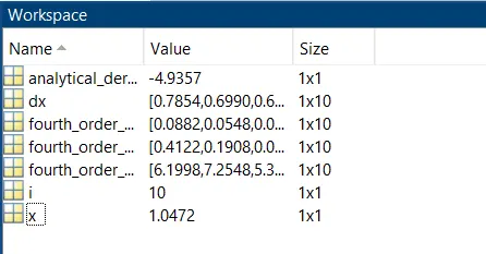
I think there is nothing to explain the above regarding the output array variables as well as the assigned variables that I explained earlier during the explanation of the functions.
So now, it's time to compare the output error variables that we have after calling the functions, & to compare with the 'dx' which is the distance between the grid size in the case of 2-D or mesh size in the case of the 3-D system.
This comparison is done by plotting the curves between the 'dx' vs the 'errors' corresponding to our derived numerical schemes as follows:
% plotting under the logarithmic scale so that plot can be visualise over
% a small region of 'dx' in an enlarged manner
loglog(dx,fourth_order_error_c,'LineWidth',1,'marker','diamond')
hold on
loglog(dx,fourth_order_error_s_r,'color','black','linewidth',1,'marker','square')
loglog(dx,fourth_order_error_s_l,'color','r','linewidth',1,'marker','o')

% for labelling/naming the X & Y axes respectively
xlabel('dx')
ylabel('errors')

% Specifying each of the curve by its name in a plotting sequence
legend('central difference of 4th order','skewed right-sided difference of 4th order','skewed left-sided difference of 4th order')

% To give title to the plot
title('Consistency of the different schemes')
We use the logarithmic plot in order to visualize the close points in a better way of the three curves that are very close to each other by enlarging the curve view that will not be better to visualize in the case of the cartesian coordinates.
So, I created three plots using the 'loglog()' command & all the plots are of the fourth order error curve w.r.t. the 'dx' as you can see in the above plotting section.
As usual I label the X & the Y-axis using the commands 'xlabel()' & 'ylabel()' respectively.
To distinguish the curves with the curve names, I use the color codes with their names using the command 'legend()' as you can see in the above plotting section.
At last, I use an additional command that is the 'title()' command in order to give a title to our logarithmic plot as you can see in the above plotting section.
Now, after running the code, I got a plot in the figure window as an output as shown below in the following screenshot:
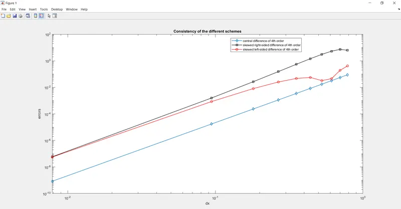
Now, I am going to explain the rate of change of the 4th orders of the errors as you can see above, w.r.t. the 'dx' as follows:
As the value of the 'dx' increases, the errors of our derived numerical schemes also increase. In that, the central order of the 4th order is lower than the skewed difference of the 4th orders i.e.,
Central difference of 4th order
As we can see from the above plot that the slope of the curve of the central difference of the 4th order is constant throughout the range of 'dx' but it changes for the skewed left-sided difference & the skewed right-sided difference of the 4th order.
Also, the error curves of the skewed difference of 4th order start from the very near about points as of (5.57*10^-8) for the skewed left-sided difference of 4th order & (5.86*10^-8) for the skewed right-sided difference of the 4th order & the difference between these points is lesser than that of (0.3).
The slope of the Central difference of 4th order is constant because the change in this is very lower in the equal units of distances in the range of 'dx'.
Now, let's discuss the portion of 'dx' from the start, (7.8*10^-3) to (9.4*10^-2):
For the central difference of 4th order, the corresponding error is from (8.41*10^-10) to (1.73*10^-5), from my point of view it is fine as the endpoint & the start point difference of the 'dx' for this portion is also high that's why we got the higher difference in the corresponding errors also as their slope may be constant, but the errors are not.
`slope=(y2-y1)/(x2-x1)`
x2=(9.4*10^-2) & x1=(7.8*10^-3)
y2=(1.73*10^-5) & y1=(8.41*10^-10)
`slope=((1.73*10^-5)-(8.41*10^-10))/((9.4*10^-2)-(7.8*10^-3))`
slope= 2.0069e-04
For the skewed left-sided difference of 4th order, the corresponding error is from (5.57*10^-8) to (0.000849132), from my point of view it is fine as the endpoint & the start point difference of the 'dx' for this portion is also high that's why we got the higher difference in the corresponding errors also as their slope may be constant, but the errors are not.
`slope=(y2-y1)/(x2-x1)`
x2=(9.4*10^-2) & x1=(7.8*10^-3)
y2=(0.000849132) & y1=(5.57*10^-8)
`slope=((0.000849132)-(5.57*10^-8))/((9.4*10^-2)-(7.8*10^-3))`
slope= 0.0099 which is more than the central difference of the 4th order so the consistency of the central difference of the 4th order is more than the consistency of the skewed left-sided difference of the 4th order.
For the skewed right-sided difference of 4th order, the corresponding error is from (5.86*10^-8) to (0.00157909), from my point of view it is fine as the endpoint & the start point difference of the 'dx' for this portion is also high that's why we got the higher difference in the corresponding errors also as their slope may be constant, but the errors are not.
`slope=(y2-y1)/(x2-x1)`
x2=(9.4*10^-2) & x1=(7.8*10^-3)
y2=(0.00157909) & y1=(5.86*10^-8)
`slope=((0.00157909)-(5.86*10^-8))/((9.4*10^-2)-(7.8*10^-3))`
slope= 0.0183 which is more than the central difference of the 4th order as well as the skewed left-sided difference of the 4th order so the consistency of the central difference of the 4th order is greatest than the consistency of the skewed left-sided difference of the 4th order as well as the skewed right-sided difference of 4th order.
Now, let's discuss the portion of 'dx' from the start, (0.094) to (0.180):
For the central difference of 4th order, the corresponding error is from (1.73*10^-5) to (23.43*10^-5), we got the higher difference in the corresponding errors but their slope may be constant, but the errors are not.
`slope=(y2-y1)/(x2-x1)`
x2=(0.180) & x1=(0.094)
y2=(23.43*10^-5) & y1=(1.73*10^-5)
`slope=((23.43*10^-5)-(1.73*10^-5))/((0.180)-(0.094))`
slope= 0.0025 which is higher than the previous range of 'dx' so now, we can say that the slope is not constant.
For the skewed left-sided difference of 4th order, the corresponding error is from (8.4*10^-4) to (8.03*10^-3), we got the lower difference in the corresponding errors which is about (0.008) also as their slope may be constant, but the errors are not.
`slope=(y2-y1)/(x2-x1)`
x2=(0.180) & x1=(0.094)
y2=(8.03*10^-3) & y1=(8.4*10^-4)
`slope=((8.03*10^-3)-(8.4*10^-4))/((0.180)-(0.094))`
slope= 0.0836 which is more than the previous range of 'dx' so now, we can say that the slope is not constant.
For the skewed right-sided difference of the 4th order, the corresponding error is from (0.0015) to (0.0266), we got the lower difference in the corresponding errors of about (0.02) & their slope may be constant, but the errors are not.
`slope=(y2-y1)/(x2-x1)`
x2=(0.180) & x1=(0.094)
y2=(0.0266) & y1=(0.0015)
`slope=((0.0266)-(0.0015))/((0.180)-(0.094))`
slope= 0.2919 which is more than the previous range of 'dx' so now, we can say that the slope is not constant.
In this manner, the curves move forwards so, in the conclusion of the explanation of this plot, I can say that the central difference of the 4th order has the least error as compared to the skewed differences of the 4th order & also the consistency of the central difference of 4th order is also more than the skewed differences of the 4th order.
The skewed differences of the 4th order may be unstable rather than the central difference of the 4th order.
The skewed scheme is useful as well as advantageous over the central difference scheme as follows:
(i). As it is less dissipative
(ii). It does not lead to oscillation in the solution or divergence if the local peclet number is larger than 2.
So I completed all your objectives as:
1. Derived the required numerical schemes.
2. Proved the 4th-order accuracy of the derived numerical schemes.
3. Evaluated the analytical function exp(x)*cos(x) using the derived numerical schemes.
4. Provides the plot as an output for comparing the errors of the derived numerical schemes in evaluating the analytical function exp(x)*cos(x).
5. And at last, the uses & advantages of the skewed schemes over the central difference schemes.
So with the completion of the all above objectives, I am going to submit this challenge.