Week 4.1 - Genetic Algorithm
AIM
- To expalin the concept of genetic algorithm and also explain the syntax for ga in MATLAB
- To write a code in MATLAB to optimise the stalagmite function and find the global maxima of the function.
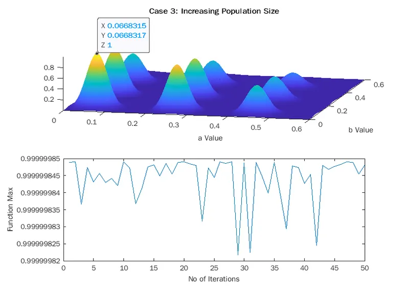
- To plot graphs for all 3 studies and for F maximum vs no. of iterations.
THEORY
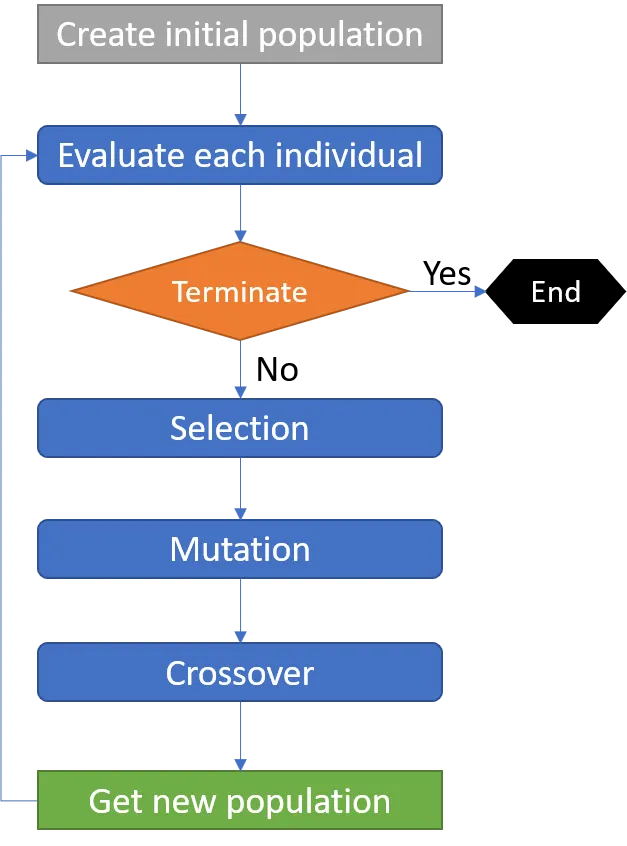
A genetic algorithm is a search heuristic that is inspired by Charles Darwin’s theory of natural evolution. This algorithm reflects the process of natural selection where the fittest individuals are selected for reproduction in order to produce offspring of the next generation. Genetic algorithms are based on the ideas of natural selection and genetics. These are intelligent exploitation of random search provided with historical data to direct the search into the region of better performance in solution space. They are commonly used to generate high-quality solutions for optimization problems and search problems.
Genetic algorithms simulate the process of natural selection which means those species who can adapt to changes in their environment are able to survive and reproduce and go to next generation. In simple words, they simulate survival of the fittest among individual of consecutive generation for solving a problem. Each generation consist of a population of individuals and each individual represents a point in search space and possible solution. Each individual is represented as a string of character/integer/float/bits. This string is analogous to the Chromosome.
Genetic algorithms are based on an analogy with genetic structure and behavior of chromosomes of the population. Following is the foundation of GAs based on this analogy –
- Individual in population compete for resources and mate
- Those individuals who are successful (fittest) then mate to create more offspring than others
- Genes from “fittest” parent propagate throughout the generation, that is sometimes parents create offspring which is better than either parent.
- Thus each successive generation is more suited for their environment.
Optimization
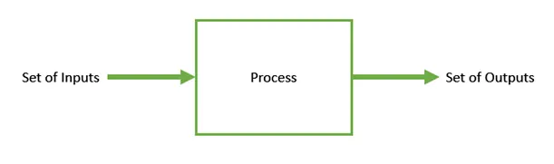
Optimization is the process of making something better. In any process, we have a set of inputs and a set of outputs as shown in the following figure. Optimization refers to finding the values of inputs in such a way that we get the best output values. The definition of best varies from problem to problem, but in mathematical terms, it refers to maximizing or minimizing one or more objective functions, by varying the input parameters.
The set of all possible solutions or values which the inputs can take make up the search space. In this search space, lies a point or a set of points which gives the optimal solution. The aim of optimization is to find that point or set of points in the search space.
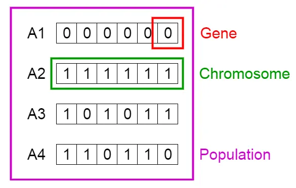
Search Space: The population of individuals are maintained within search space. Each individual represents a solution in search space for given problem. Each individual is coded as a finite length vector (analogous to chromosome) of components. These variable components are analogous to Genes. Thus a chromosome (individual) is composed of several genes (variable components).
Fitness Score: A Fitness Score is given to each individual which shows the ability of an individual to compete. The individual having optimal fitness score (or near optimal) are sought.
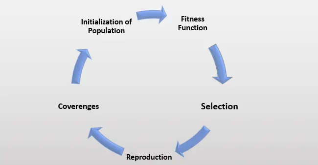
Five phases are considered in a genetic algorithm.
- Initial population
- Fitness function
- Selection
- Crossover
- Mutation
Initial Population : The process begins with a set of individuals which is called a Population. Each individual is a solution to the problem you want to solve. An individual is characterized by a set of parameters (variables) known as Genes. Genes are joined into a string to form a Chromosome (solution). In a genetic algorithm, the set of genes of an individual is represented using a string, in terms of an alphabet. Usually, binary values are used (string of 1s and 0s). We say that we encode the genes in a chromosome.
Fitness Function
The fitness function determines how fit an individual is (the ability of an individual to compete with other individuals). It gives a fitness score to each individual. The probability that an individual will be selected for reproduction is based on its fitness score.
Selection
The idea of selection phase is to select the fittest individuals and let them pass their genes to the next generation. Two pairs of individuals (parents) are selected based on their fitness scores. Individuals with high fitness have more chance to be selected for reproduction.
Crossover
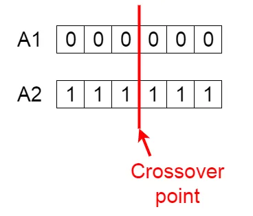
Crossover is the most significant phase in a genetic algorithm. For each pair of parents to be mated, a crossover point is chosen at random from within the genes. For example, consider the crossover point to be 3 as shown below.
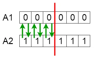
Offspring are created by exchanging the genes of parents among themselves until the crossover point is reached.
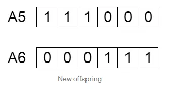
The new offspring are added to the population.
Mutation
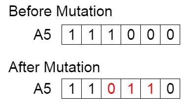
In certain new offspring formed, some of their genes can be subjected to a mutation with a low random probability. This implies that some of the bits in the bit string can be flipped. Mutation occurs to maintain diversity within the population and prevent premature convergence.
Advantages Of GA's
GAs have various advantages which have made them immensely popular. These include
- Does not require any derivative information (which may not be available for many real-world problems).
- Is faster and more efficient as compared to the traditional methods.
- Has very good parallel capabilities.
- Optimizes both continuous and discrete functions and also multi-objective problems.
- Provides a list of “good” solutions and not just a single solution.
- Always gets an answer to the problem, which gets better over the time.
- Useful when the search space is very large and there are a large number of parameters involved.
Disadvantages Of GA's
Like any technique, GAs also suffer from a few limitations. These include
- GAs are not suited for all problems, especially problems which are simple and for which derivative information is available.
- Fitness value is calculated repeatedly which might be computationally expensive for some problems.
- Being stochastic, there are no guarantees on the optimality or the quality of the solution.
- If not implemented properly, the GA may not converge to the optimal solution.
Applications
Genetic algorithms have many applications, some of them are
- Recurrent Neural Network
- Mutation testing
- Code breaking
- Filtering and signal processing
- Learning fuzzy rule base etc
Traditional calculus based methods work by starting at a random point and by moving in the direction of the gradient, till we reach the top of the hill. This technique is efficient and works very well for single-peaked objective functions like the cost function in linear regression. But, in most real-world situations, we have a very complex problem called as landscapes, which are made of many peaks and many valleys, which causes such methods to fail, as they suffer from an inherent tendency of getting stuck at the local optima
Some difficult problems like the Travelling Salesperson Problem (TSP), have real-world applications like path finding and VLSI Design. Now imagine that you are using your GPS Navigation system, and it takes a few minutes (or even a few hours) to compute the optimal path from the source to destination. Delay in such real world applications is not acceptable and therefore a good-enough solution, which is delivered fast is what is required.
Syntax
- x = ga(fun,nvars)
- x = ga(fun,nvars,A,b)
- x = ga(fun,nvars,A,b,Aeq,beq)
- x = ga(fun,nvars,A,b,Aeq,beq,lb,ub)
- x = ga(fun,nvars,A,b,Aeq,beq,lb,ub,nonlcon)
- x = ga(fun,nvars,A,b,Aeq,beq,lb,ub,nonlcon,options)
- x = ga(fun,nvars,A,b,Aeq,beq,lb,ub,nonlcon,intcon)
- x = ga(fun,nvars,A,b,Aeq,beq,lb,ub,nonlcon,intcon,options)
- x = ga(problem)
- [x,fval] = ga(___)
- [x,fval,exitflag,output] = ga(___)
- [x,fval,exitflag,output,population,scores] = ga(___)
where x is local minima input
fun - function to be called (here stalagmite function)
nvars - number of variables used
A,b,Aeq,beq - Inequalities in the function
lb - lower bound
ub - upper bound
nonlcon - vector of non linear constraints (accepts an arrary or a vector and returns two arrays)
intcon - Vector of integer constraints
options - perform additional operations
Function Used
`f(x,y) = underset(1,x)(f)` `underset(2,x)(f)` `underset(1,y)(f)` `underset(2,y)(f)`
`underset(1,x)(f) = [sin(5.1pix+0.5)]^6`
`underset(1,y)(f) = [sin(5.1piy+0.5)]^6`
`underset(2,x)(f) = exp[-4ln(2)(x-0.0667)^2/0.64]`
`underset(2,y)(f) = exp[-4ln(2)(y-0.0667)^2/0.64]`
PROGRAMMING LANGUAGE
Matlab
ALGORITHM
Functions
- Start
- Creating a function which can take inputs and give output
- Intialize the variable
- Allocating the equations into four different varaibles
- Solving the function using the specified equation by defining the function (to get the max value we are giving negative sign).
- Exit
Main Program
- Start
- Define the search space by using linspace command and assign it to different variables
- Define the number of cases the loop to be iterated
- Create a 2D array by using meshgrid command.
- Evalute the stalagmite function by calling the function using for loop
- Plot a 3d graph using surfc command.
- Repeat the steps for 3 cases -
1. without boundary condition
2. With Boundary Condition
3. By increasing population size
- Plot 'Function Max vs No of Iteration' graph for each case
- Exit
PROGRAM
Function
%creating a function whichcan take inputs
function [f] = stalagmite(ip_v)
%initializing the variables
a = ip_v(1);
b = ip_v(2);

%allocating the equation to 4 variables
tm1 = (sin((5.1*pi*a)+0.5))^6;
tm2 = (sin((5.1*pi*b)+0.5))^6;
tm3 = exp(-4*log(2)*((a-0.0667)^2)/(0.64));
tm4 = exp(-4*log(2)*((b-0.0667)^2)/(0.64));

%defining the function
f = -(tm1*tm2*tm3*tm4);
end
Main Program
%Program to optimise the stalagmite function and
% find the global maxima of the function
clear all
close all
clc
%defining the search space by using linspace command
a = linspace(0,0.6,150);
b = linspace(0,0.6,150);
%defining no of cases
n = 50;
%Creating a 2D array using Meshgrid
[aa, bb] = meshgrid(a,b);

%Evaluating the stalagmite function
for i=1:length(aa)
    for j=1:length(bb)
        ip_v(1) = aa(i,j);
        ip_v(2) = bb(i,j);
        f(i,j) = stalagmite(ip_v);  %Calling the function
    end
end

%Plotting
figure(1)
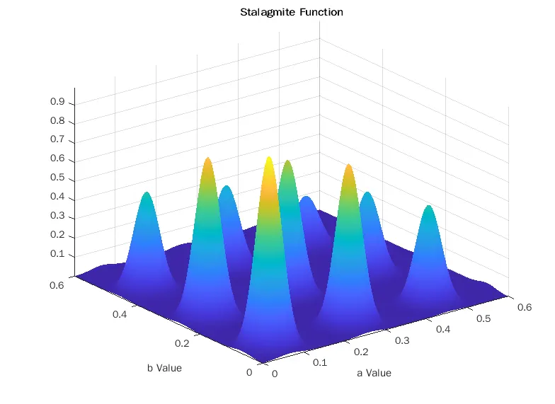
surfc(aa,bb,-f);  % -ve sign to get max value
shading interp;   %to get plot smoother and without grid
xlabel('a Value');
ylabel('b Value');
title('Stalagmite Function');

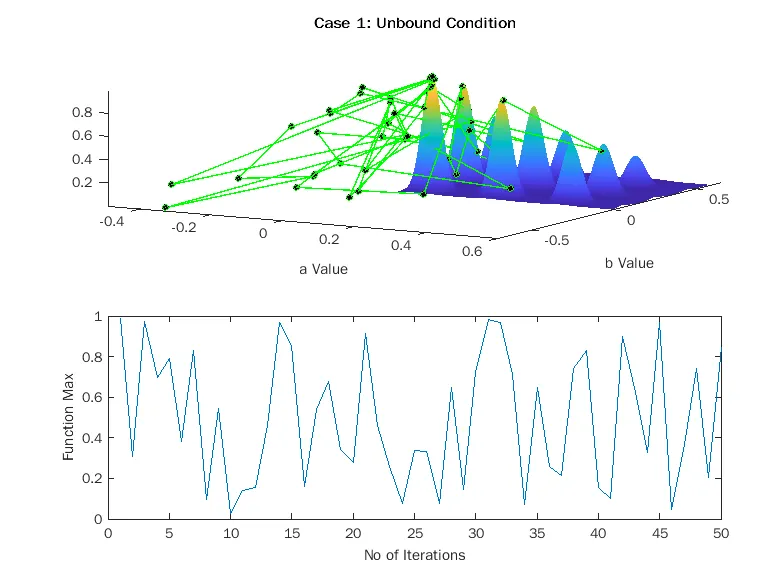
%Case 1: Statistical Behaviour without boundary condition
tic    %to get how much time taken to compile the code
for i=1:n
[ip,fot(i)] = ga(@stalagmite,2);
aot(i) = ip(1);
bot(i) = ip(2);
end
case1 = toc

%Plotting
figure(2)
subplot(2,1,1);
hold on
surfc(aa,bb,-f);
shading interp;
xlabel('a Value');
ylabel('b Value');
title('Unbound Condition');

plot3(aot,bot,-fot,'linewidth',1,'color','g','marker','o','markersize',5,'markerfacecolor','k');
subplot(2,1,2);
plot(-fot);
xlabel('No of Iterations');
ylabel('Function Max');

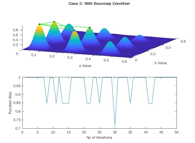
%Case 2: Statistical Behaviour with boundary condition
tic
for i=1:n
[ip,fot(i)] = ga(@stalagmite,2,[],[],[],[],[0;0],[0.6;0.6]);
aot(i) = ip(1);
bot(i) = ip(2);
end
case2 = toc

%Plotting
figure(3)
subplot(2,1,1);
hold on
surfc(aa,bb,-f);
shading interp;
xlabel('a Value');
ylabel('b Value');
title('With Boundary Condition');

plot3(aot,bot,-fot,'linewidth',1,'color','g','marker','o','markersize',5,'markerfacecolor','k');
subplot(2,1,2);
plot(-fot);
xlabel('No of Iterations');
ylabel('Function Max');

%Case 3: Statistical Behaviour by Increasing Population size
ot = optimoptions('ga');
ot = optimoptions(ot,'PopulationSize',400);
tic
for i=1:n
[ip,fot(i)] = ga(@stalagmite,2,[],[],[],[],[0;0],[0.6;0.6],[],[],ot);
aot(i) = ip(1);
bot(i) = ip(2);
end
case3 = toc

%Plotting
figure(4)
subplot(2,1,1);
hold on
surfc(aa,bb,-f);
shading interp;
xlabel('a Value');
ylabel('b Value');
title('Increasing Population Size');

plot3(aot,bot,-fot,'linewidth',1,'color','g','marker','o','markersize',5,'markerfacecolor','k');
subplot(2,1,2);
plot(-fot);
xlabel('No of Iterations');
ylabel('Function Max');
ERRORS OCCURED
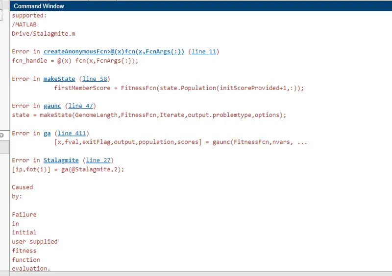
Corrections Done: Gone through the syntax once more and made corrections like spelling mistake, closing parenthesis etc
OUTPUT
Case 1
Case 2
Case 3
CONCLUSION
- The concept of genetic algorithm with syntax has been explained.
- Program to optimise the stalagmite function and find the global maxima of the given function has been run successfully.
- Plotted graphs for all 3 studies.
REFERENCE
https://skill-lync.com/knowledgebase/genetic-algorithm-explained
https://en.wikipedia.org/wiki/List_of_genetic_algorithm_applications
https://en.wikipedia.org/wiki/Genetic_algorithm
https://www.tutorialspoint.com/genetic_algorithms/genetic_algorithms_introduction.htm