Week 3 - Solving second order ODEs

AIM

• To write a program that solves the given Ordinary Differential Equation (ODE) that represents the equation of motion of a simple pendulum with damping
• To write a program in Matlab\Octave that will simulate the pendulum motion

THEORY

Ordinary Differential Equation: An ordinary differential equation is an equation which consists of one or more functions of one independent variable along with their derivatives. A differential equation is an equation that contains a function with one or more derivatives. But in the case ODE, the word ordinary is used for derivative of the functions for the single independent variable.

Simple Pendulum: A simple pendulum is a mechanical arrangement that demonstrates periodic motion. The simple pendulum comprises a small bob of mass, suspended by a thin string secured to a platform at its upper end of length. When a pendulum is displaced sideways from its resting, equillibrium position, it is subject to a restoring force due to gravity that will accelerate it back toward the equilibrium position. When released, the restoring force acting on the pendulum's mass causes it to oscillate about the equilibrium position, swinging back and forth. The time for one complete cycle, a left swing and a right swing, is called the period. The period depends on the length of the pendulum and also to a slight degree on the amplitude, the width of the pendulum's swing.

• The oscillatory motion of a simple pendulum: Oscillatory motion is defined as the to and fro motion of the pendulum in a periodic fashion and the centre point of oscillation known as equilibrium position.
• The time period of a simple pendulum: It is defined as the time taken by the pendulum to finish one full oscillation.
• The amplitude of simple pendulum: It is defined as the distance travelled by the pendulum from the equilibrium position to one side.
• Length of a simple pendulum: It is defined as the distance between the point of suspension to the centre of the bob.

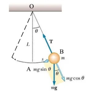
The ODE represents the equation of motion of a simple pendulum with damping is given by

`(d^2theta)/dt^2 + b/m (d theta)/dt + g/L sin theta = 0`

where

g = gravity in `m/s^2`,

L = length of the pendulum in m,

m = mass of the ball in kg,

b=damping coefficient.

According to Newton's Second Law,

`(d^2theta)/dt^2 + b/m (d theta)/dt + g/L sin theta = 0`

Let `theta = underset(1)(theta)`

so equation becomes `(d^2underset(1)(theta))/dt^2 + b/m (d underset(1)(theta))/dt + g/L sin underset(1)(theta) = 0`

`(d theta)/dt = (dunderset(1)(theta))/dt = underset(2)(theta)`

`(d^2 theta)/dt^2 = (d^2 underset(1)(theta))/dt^2 = d/dt((dunderset(1)(theta))/dt) = (dunderset(2)(theta))/dt`

Substituting all these values in main equation, so main equation becomes

`(dunderset(2)(theta))/dt + b/m underset(2)(theta) + g/L sinunderset(1)(theta) = 0`

`(dunderset(1)(theta))/dt = underset(2)(theta)`

`(dunderset(2)(theta))/dt = -b/m underset(2)(theta) - g/L sin underset(1)(theta)`

`d/dt [[underset(1)(theta)] , [underset(2)(theta)]]` = `[[underset(2)(theta)] , [-b/m underset(2)(theta) - g/L sin underset(1)(theta)]]`

This second order ODE equation can be used to solve the simple pendulum.

PROGRAMMING LANGUAGE

Matlab

ALGORITHM

Main Program

• Start
• Clear the workspace, close all the figures and plots, clear the command window
• Initialize the input parameters like damping coefficient, acceleration due to gravity, length of the pendulum, mass of the ball/bob
• Assume ang. Displacement as 0 and ang. Velocity as 3 at time 0 as initial condition.
• Create an array for time using linspace command.
• Solve the ODE by calling the function
• Print Ang. Displacement and Ang. Velocity.
• Plot Ang. Displacement vs Time and Ang. Velocity vs Time graph
• Create a for loop for animation of pendulum and define the respective coordinates
• Plot for rigid support, point of suspension, length of pendulum, ball.
• Define the axis
• Capture each plot by using getframe command
• Create a movie file in avi format
• Exit

Function

• Start
• Creating a function that depend on angle and time which can take inputs and give output.
• Define each terms in the ODE as per the theoretical solution
• Defining the function such that it’s output would be a matrix.
• End

PROGRAM

Main Program

%Program to solve program that solves the Ordinary Differential Equation (ODE)
% that represents the equation of motion of a simple pendulum with damping
clear all 
close all
clc

%inputs
b = 0.05; %Damping Coefficient
g = 9.81; %acceleration due to gravity
l = 1;    %length of the pendulum
m = 1;    %mass of the ball
%intial assumption of ang.displacement as 0, and ang. velocity as 5
initial_cond = [0;3]; 
%creating an array for time using linspace command 
ts = linspace(0,20,500);
%calling the function to find the solution of ODE
[time,ans] = ode45(@(time,angle)pendulum_fun(angle,time,b,g,l,m),ts,initial_cond);
disp = ans(:,1);
vel = ans(:,2);

%Plotting
%Plotting Ang.Displacement VS Time
figure(1)
plot(time,disp,'LineWidth',1.5,'color','b');
xlabel('Time [s]');
ylabel('Angular Displacement [rad]')
title('Ang.Displacement VS Time')

%Plotting Ang.Velocity VS Time
figure(2)
plot(time,vel,'LineWidth',1.5,'color','m')
xlabel('Time [s]');
ylabel('Angular Velocity [rad/s]')
title('Ang.Velocity VS Time')

%Plotting Ang. Displacement, Ang.Velocity VS Time
figure(3)
hold on
plot(time,disp,'LineWidth',1.5,'color','b')
plot(time,vel,'LineWidth',1.5,'color','m')
title('Ang.Displacement & Ang. Velocity VS Time Combined')
xlabel('Time [s]')
ylabel('Ang.Displacement / Ang. Velocity')
legend('Ang.Displacement', 'Ang.Velocity')


%Creating the animation of the pendulum    
ct = 1;  %counter for incrementing the value in every iteration of for loop

for i=1:length(disp)
    mot=disp(i);
    x0=0;
    y0=0;
    x1=l*sin(mot);
    y1=-l*cos(mot);
    
    figure(4)
    
   %Plotting rigid support
   plot([-1 1], [0 0],'LineWidth',3,'color','b');
   hold on
   %Plotting for point of suspension
   plot(x0,y0,'o','MarkerFaceColor','y','MarkerSize',6)
   %For length of pendulum
   plot([x0 x1],[y0 y1],'color','r')
   %For bob/ball
   plot(x1,y1,'o','MarkerFaceColor','k','MarkerSize',20)
   hold off 
   axis([-2 2 -2 2])   %defining the axis
   legend('Rigid Support','Point Of Suspension','Length of Pendulum','Bob')
   pause(0.001)
    M(ct) = getframe(gcf);   %capturing current figure
    ct=ct+1;
end

%creating the movie file in avi format
movie(M)
anim = VideoWriter('Pendulum.avi','Uncompressed AVI');
open(anim);
writeVideo(anim,M);
close(anim);

Function

%function to solve the ODE of pendulum
%creating a function with inputs
function [dangle_dt] = pendulum_fun(angle,time,b,g,l,m)
angle1 = angle(1);
angle2 = angle(2);
dangle1_dt = angle2;
dangle2_dt = (-b/m)*angle2-(g/l)*sin(angle1);
%defining the function
dangle_dt = [dangle1_dt;dangle2_dt];
end

ERRORS OCCURED

• The values of X1 and Y1 are wrongly specified.

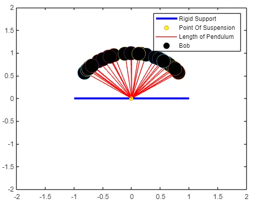
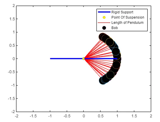
Correction Done: Values are specified correctly and give a negative sign.

• Improper Placing of hold on command always thrown error throughout the running of program

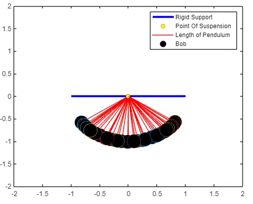
Coorection Done: Tried hold on and hold off comand a lot of time in many places until the figure comes perfectly.

OUTPUT

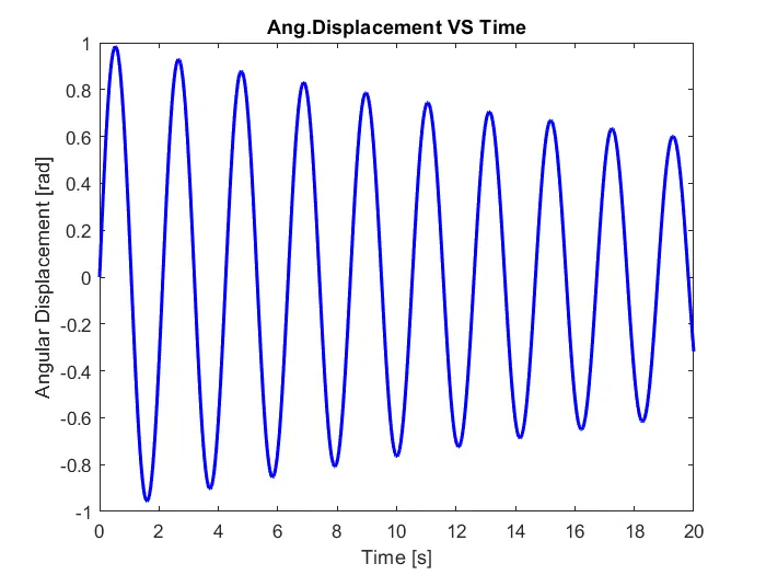
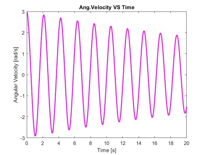
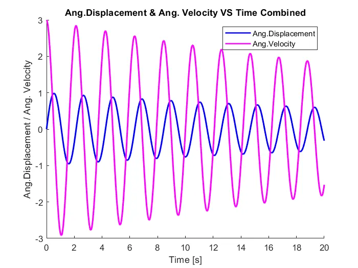
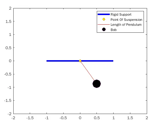
The animation of the pendulum can be seen by clicking the link below

https://drive.google.com/file/d/1Cgv006uhz5AkHnBRpQ20JbXSZs9dZSvp/view?usp=sharing

CONCLUSION

• Program that solves the given Ordinary Differential Equation (ODE) that represents the equation of motion of a simple pendulum with damping has been run successfully.
• Simulation of the pendulum motion has been successfully carried out in Matlab and created a google drive link.