Project 2 - Rankine cycle Simulator

AIM

• To create a Rankine Cycle Simulator using MATLAB and to calculate the state points based on user inputs
• To plot the corresponding T-s and h-s plots for the given set of inputs.

THEORY

RANKINE CYCLE

We know that the Carnot cycle is most efficient cycle operating between two specified temperature limits. However, the Carnot cycle is not a suitable model for steam power cycle since:

• The turbine has to handle steam with low quality which will cause erosion and wear in turbine blades.
• It is impractical to design a compressor that handles two phase.
• It is difficult to control the condensation process

Other issues include: isentropic compression to extremely high pressure and isothermal heat transfer at variable pressures. Thus, the Carnot cycle cannot be approximated in actual devices and is not a realistic model for vapor power cycles.

The Rankine cycle has become the go to process in the vapor power plants. In contrast to the Carnot cycle, this method of power generation provides more value to the outcome of the process. Its ability to increase the working temperature, providing high-quality steam with less moisture content to the turbine, and much easier handling of steam and water are some of the positives that contribute to the overall efficiency of the process.

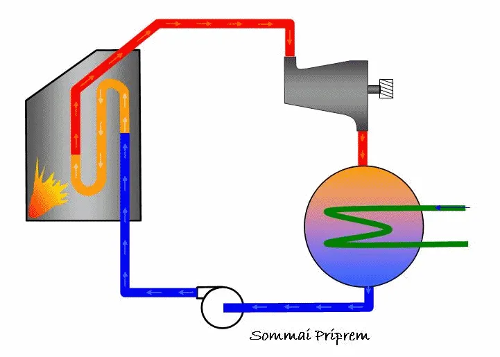
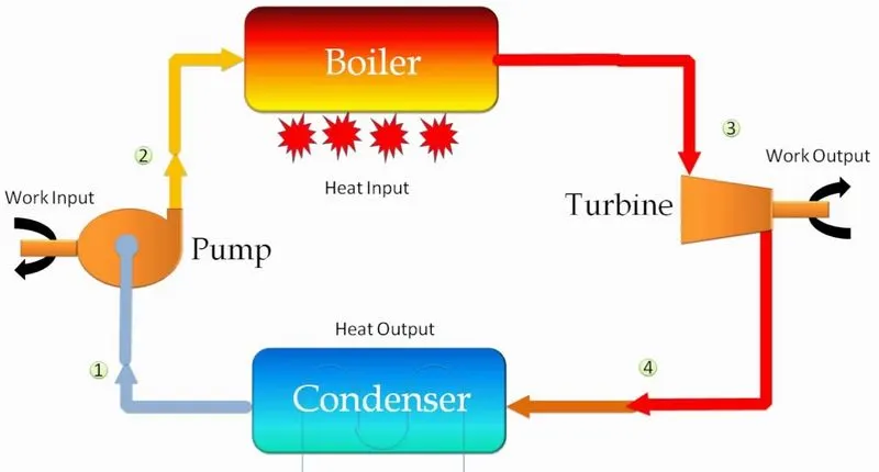
Usually, a power plant consists of four major components in general. They are a feed pump, Boiler, Turbine, and Condenser. Rankine cycle reveals the state of water, Working temperature, and pressure, entropies, and enthalpies at each stage of the closed-loop process.

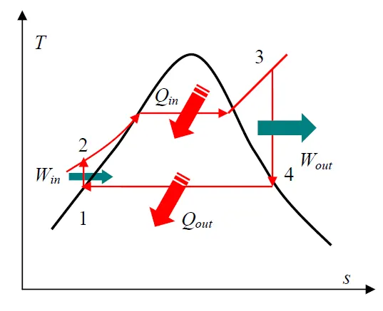
The ideal cycle consists of 4 major processes and each of them is reversible processes.

• 1-2 Isentropic Compression in the Feed Pump

Water enters the pump as state 1 as saturated liquid and is compressed isentropically to the operating pressure of the boiler.

• 2-3 Constant Pressure Heat Addition in the Boiler

Saturated water enters the boiler and leaves it as superheated vapor.

• 3-4 Isentropic Expansion in the Turbine

Superheated vapor expands isentropically in turbine and produces work.

• 4-1 Constant Pressure Heat Removal in the Condenser

High quality steam is condensed in the condenser

Working Of Ideal Rankine Cycle

Saturated water from state 1 will enter the feed pump. The feed pump will compress the saturated liquid isentropically to the operating pressure of the boiler. The temperature of the liquid will increase marginally and by now the liquid has shifted from saturating level to a compressed state. Thereafter compressed liquid from sate 2 will head to the boiler. Here the liquid will transform to superheated steam at a constant pressure. As a result of this, the temperature of the steam will increase drastically. Then superheated steam from state 3 will go past the turbines to produce work. This an isentropic where the pressure and the temperature will decrease considerably. At the end of the process, steam has now become a liquid-vapor mixture. Finally, the mixture from stage 4 will go through the condenser to produce saturated liquid in a constant pressure process.

ACTUAL RANKINE CYCLE

It is impossible to achieve ideal conditions in vapor power plants. So, there is always a dip in efficiency in real situations. Fluid friction is one such effect that creates inefficiencies in the cycle. This will lead to pressure losses in the boiler and the condenser. A pressure drop in the boiler will result in low-pressure steam to the turbine which decreases the work output. As a result of pressure loss in the turbine, the feed pump will require a little more work input than the anticipated input. The other major cause of concern is heat losses throughout the cycle. This will result in more energy requirements than ideal conditions.

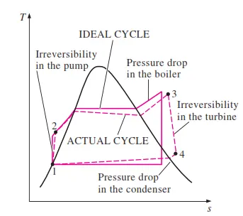
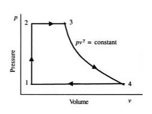
The actual Rankine cycle T-S diagram is very much similar to that of the ideal cycle except for a few variations. Here Pump and the turbine will not act isentropically. The pump will require more work in and the turbine results in low work out. These two processes aren’t reversible anymore. Hence the entropy of the following stages will have higher entropy.

The feed pump will elevate the pressure of the saturated liquid in the process related to state 1 to state 2. There is no change in volume in the process. State 2 to state 3 is a constant pressure process. Since liquid converts to steam, the volume of the system will increase considerably. State 3 to state 4 is an isentropic expansion process. As the name suggests the volume of the system will increase and pressure drop occurs as it passes through the turbine. The final step which is stage 4 to 1 occurs in the condenser with no pressure drop. As the saturated steam converts to the saturated liquid, the volume of the system will decrease considerably

Rankine Cycle Thermal Efficiency

All four components of the Rankine cycle are steady-state steady-flow devices.

The Steady Flow Energy Equation is given by:

`underset(1)(h) + (underset(1)(c)^2)/2 + gunderset(1)(z) + dot Q = underset(2)(h) + (underset(2)(c)^2)/2 + gunderset(2)(z) + dot W`

Where `underset(1)(h)`, `underset(2)(h)` are enthalpies at inlet and outlet

`(underset(1)(c)^2)/2`, `(underset(2)(c)^2)/2` are Kinetic Energies

`gunderset(1)(z)`, `gunderset(2)(z)` are Potential Energies

`dot Q` is the heat added/rejected per unit time

`dot W` is the work done per unit time

The potential and kinetic energy effects can be neglected. Considering the isentropic behavior in an ideal cycle,

Work Done by Pump, `underset(p)(W)` = `underset(2)(h)` - `underset(1)(h)`

Heat Added to the Boiler, `underset(i n)(Q)`= `underset(3)(h)` - `underset(2)(h)`

Work Done by Turbine, `underset(T)(W)` = `underset(3)(h)` - `underset(4)(h)`

Heat rejected from the Condenser, `underset(out)(Q)`= `underset(4)(h)` - `underset(1)(h)`

Thermal efficiency is defined as the ratio of net work done to the heat added. it is denoted by `underset(th)(eta)`.

`underset(th)(eta)` = `underset(n et)(W)/ underset(i n)(Q)`

`underset(n et)(W) = underset(i n)(Q) - underset(out)(Q)`

so, `underset(th)(eta)` = `(underset(i n)(Q) - underset(out)(Q))/underset(i n)(Q)`

Steam Rate

Steam rate is defined as the ratio of amount of steam(kg) or steam flow in Kg/hr required to produce unit shaft power output (1KW). It is a measure of the capacity of a power plant The unit is Kg/KWh. Higher steam rate implies more steam consumption for particular amount of power, hence lower steam rate is desirable for a power plant

Steam Rate = `3600/underset(n et)(W)` `((Kg)/(KWh))`

Heat Rate

Heat rate is the rate of heat input in KJ/hr to produce unit power of 1KW. It indicates the amount of fuel required to generate one unit of electricity. It is expressed in KJ/KW-hr

Heat Rate = `(3600 times underset(i n )(Q))/underset(n et)(W)` `((KJ)/(KW-hr))`

Work Ratio

Work Ratio is defined as net work output of the cycle to the work developed by the turbine

Work Ratio, `WR = (underset(n et)(W))/ underset(T)(W)`

Back Work Ratio

Back work ratio is defined as pump work input to work developed by turbine

Back Work Ratio, `underset(back)(WR) = (underset(p)(W))/ underset(T)(W)`

Dryness Fraction

The steam dryness fraction is used to quantify the amount of water within steam. If steam contains 10% water by mass, it's said to be 90% dry, or have a dryness fraction of 0.9. Steam dryness is important because it has a direct effect on the total amount of transferable energy contained within the steam (usually just latent heat), which affects heating efficiency and quality. Steam tables contain values such as enthalpy (h), specific volume (ν), entropy (s), etc. for saturated steam (100% dry) and for saturated water (0% dryness), but typically not for wet steam.

Specific enthalpy of wet stream is given by:

`h = underset(f)(h) + X. underset(fg)(h)`

where X = Dryness

`underset(f)(h)` = Specific Enthalpy of Saturated Water

`underset(fg)(h)` = Specific Enthalpy of Saturated Steam - Specific Enthalpy of Saturated Water (`underset(g)(h) - underset(f)(h)`)

Simillarly, Specific entropy of wet stream is given by:

`s = underset(f)(s) + X. underset(fg)(s)`

where X = Dryness

`underset(f)(s)` = Specific Entropy of Saturated Water

`underset(fg)(s)` = Specific Entropy of Saturated Steam - Specific Entropy of Saturated Water (`underset(g)(s) - underset(f)(s)`)

PROGRAMMING LANGUAGE

Matlab

ALGORITHM

• Start
• Clear the work space, close all plots and figures, clear the command window.
• Print the main heading as 'Rankine Cycle Simulator'.
• Print all the processes takes place in rankine cycle.
• Define temperature, pressure as per the given criteria such that it can take user input as the value.
• Find the parameters in each state points from the given data file 'XSteam.m'.
• Find required properties such as enthalpy, entropy, temperature of each states from XSteam using basic rankine cycle relations
• Find Work done, Net work, Thermal Efficiency, Steam rate, Heat rate, Work Ratio, Back Work Ratio using specified formulas and print it as results.
• Plot T-S Diagram and H-S Diagram
• Print all the results in Command Window
• Exit

PROGRAM

clear all
close all
clc
fprintf('%s\n','---------- RANKINE CYCLE SIMULATOR ---------');
fprintf('%s\n','1-2 : Const Pressure Heat Addition by the Boiler');
fprintf('%s\n','2-3 : Isentropic Expansion in the Turbine');
fprintf('%s\n','3-4 : Const Pressure Heat Rejection by the Condenser');
fprintf('%s\n\n','4-1 : Isentropic Compression by the Pump');

%inputs
p3 = input('Value of Pressure at turbine inlet,p3 (bar) = ');
T3 = input('Value of Temperature at turbine inlet,t3 (degree C) = ');
p4 = input('Value of Pressure at condenser inlet,p4 (bar) = ');
fprintf('\n');
%extracting enthalpy and entropy value at state point 3 from XSteam
h3 = XSteam('h_pT',p3,T3);
s3 = XSteam('s_pT',p3,T3);

%state point 4 
%Extracting required datas from XSteam
s4=s3;                       %Since it is an isentropic process entropy remains const
sf4 = XSteam('sL_p',p4);     %Specific entropy of saturated water
sg4 = XSteam('sV_p',p4);     %Specific entropy of saturated steam
hf4 = XSteam('hL_p',p4);     %Specific enthalpy of saturated water
hg4 = XSteam('hV_p',p4);     %Specific enthalpy of saturated steam
x4 = (s4-sf4)/(sg4-sf4);     %Dryness
h4 = hf4 + (x4*(hg4-hf4));   %Enthalpy at point 4

%state point 1 
%Extracting required datas from XSteam
p1 = p4;                     %Since it is an isobaric process pressure remains const
s1 = XSteam('sL_p',p1);
h1 = XSteam('hL_p',p1);
T1 = XSteam('Tsat_p',p1);
T4 = T1;                    %Temperature remains const

%state point 2
s2 = s1;                    %entropy remains const
p2 = p3;                    %pressure remains const
h2 = XSteam('h_ps',p2,s2);

%extracting values for Specific heat capacity at cons pressure(Cp) and const volume(Cv)  
cp2 = XSteam('Cp_ps',p2,s2);
cv2 = XSteam('Cv_ps',p2,s2);
gamma = cp2/cv2;
T2 = ((p2/p1)^(1-(1/gamma)))*T1;

%state point 5
h5 = XSteam('hL_p',p2);
s5 = XSteam('sL_p',p2);
T5 = XSteam('T_hs',h5,s5);

%state point 6
h6 = XSteam('hV_p',p3);
s6 = XSteam('sV_p',p3);
T6 = XSteam('T_hs',h6,s6);

%for creating curve for superheated state
sc = linspace(s3,s6,600);
for m = 1:length(sc)
    Tc(m) = XSteam('T_ps',p3,sc(m));
end

%work done by turbine
wt = h3-h4;

%work done by pump
wp = h2-h1;

%Net work done
wnet = wt - wp;

%heat added to boiler
qin = h3 - h2;

%heat removed from condenser
qout = h4 - h1;

%Thermal Efficiency
E = (wnet/qin)*100;

%Steam Rate
Sr = 3600/wnet;

%Heat Rate
Hr = (3600*qin)/wnet;

%Work ratio
wr = wnet/wt;

%Back work ratio
wrb = wp/wt;

%For creating saturation dome or saturation curve
ts = linspace(1,400,650);
for i=1:length(ts);
    sat_sl(i) = XSteam('sL_T',ts(i));
    sat_sv(i) = XSteam('sV_T',ts(i));
    
    sat_hl(i) = XSteam('hL_T',ts(i));
    sat_hv(i) = XSteam('hV_T',ts(i));
end

%Plotting T-S Diagram
figure(1)
hold on
plot([s3 s4],[T3 T4],'linewidth',2.5,'Color','b');
plot([s4 s1],[T4 T1],'linewidth',2.5,'Color','g');
plot([s1 s2],[T1 T2],'linewidth',2.5,'Color','c');
plot(sat_sl,ts,'--','linewidth',1.5,'color','k')
plot([s2 s5],[T2 T5],[s5 s6],[T5 T6],sc,Tc,'linewidth',2.5,'Color','r');
text(s3+0.1,T3,'3');
text(s4+0.1,T4,'4');
text(s1+0.2,T1,'1');
text(s2-0.4,T2,'2');
text(s5-0.4,T5,'5');
text(s6+0.2,T6,'6');
plot(sat_sv,ts,'--','linewidth',1.5,'color','k')
axis([0 10 0 750]);
legend({'Isentropic Expansion in Turbine','Heat Removal in Condenser','Isentropic Compression in pump','Saturation Curve','Heat Addition in Boiler'},'Location','northwest');
title('T-S Diagram');
xlabel('Entropy [KJ/KgK]');
ylabel('Temperature [^oC]')

%Plotting H-S Diagram
figure(2)
hold on
plot([s3 s4],[h3 h4],'linewidth',2.5,'Color','b');
plot([s4 s1],[h4 h1],'linewidth',2.5,'Color','g');
plot([s1 s2],[h1 h2],'linewidth',2.5,'Color','c');
plot(sat_sl,sat_hl,'--','linewidth',1.5,'color','k')
plot([s2 s5],[h2 h5],[s5 s6],[h5 h6],[s6 s3],[h6 h3],'linewidth',2.5,'Color','r');
text(s3+0.1,h3,'3');
text(s4+0.1,h4,'4');
text(s1+0.3,h1,'1');
text(s2-0.3,h2,'2');
text(s5-0.4,h5,'5');
text(s6-0.6,h6,'6');
plot(sat_sv,sat_hv,'--','linewidth',1.5,'color','k')
legend({'Isentropic Expansion in Turbine','Heat Removal in Condenser','Isentropic Compression in pump','Saturation Curve','Heat Addition in Boiler'},'Location','northwest');
title('H-S Diagram');
xlabel('Entropy [KJ/KgK]');
ylabel('Enthalpy [KJ/Kg]');

%Printing the results
fprintf('%35s\n','RESULTS');
fprintf('%s %50s\n','At State Point 1:','At State Point 2:');
fprintf('\n%s %4.2f %s %41s %4.2f %s\n','P1 is :',p1,'Bar','P2 is :',p2,'Bar');
fprintf('%s %4.2f %s %32s %4.2f %s\n','T1 is :',T1,'Deg Celcius','T2 is :',T2,'Deg Celcius');
fprintf('%s %4.2f %s %37s %4.2f %s\n','H1 is :',h1,'KJ/Kg','H2 is :',h2,'KJ/Kg');
fprintf('%s %4.2f %s %38s %4.2f %s\n','S1 is :',s1,'KJ/KgK','S2 is :',s2,'KJ/KgK');
fprintf('\n');

fprintf('%s %50s\n','At State Point 3:','At State Point 4:');
fprintf('\n%s %4.2f %s %41s %4.2f %s\n','P3 is :',p3,'Bar','P4 is :',p4,'Bar');
fprintf('%s %4.2f %s %32s %4.2f %s\n','T3 is :',T3,'Deg Celcius','T4 is :',T4,'Deg Celcius');
fprintf('%s %4.2f %s %37s %4.2f %s\n','H3 is :',h3,'KJ/Kg','H4 is :',h4,'KJ/Kg');
fprintf('%s %4.2f %s %39s %4.2f %s\n','S3 is :',s3,'KJ/KgK','S4 is :',s4,'KJ/KgK');
fprintf('\n');

fprintf('%s %4.2f % s\n','Work Done By The Turbine, WT:',wt,'KJ/Kg');
fprintf('%s %4.2f % s\n','Work Done By The Pump, Wp:',wp,'KJ/Kg');
fprintf('%s %4.2f % s\n','Heat Added To The Boiler, Qin:',qin,'KJ/Kg');
fprintf('%s %4.2f % s\n','Heat Removed From The Condenser, Qout:',qout,'KJ/Kg');
fprintf('%s %4.2f % s\n','Net Work Done, WNet:',wnet,'KJ/Kg');
fprintf('%s %4.2f % s\n','Thermal Efficiency Of Rankine Cycle E:',E,'%');
fprintf('%s %4.2f % s\n','Steam Rate, SSC:',Sr,'Kg/KWh');
fprintf('%s %4.2f % s\n','Heat Rate, Hr:',Hr,'KJ/KWh');
fprintf('%s %f\n','Work Ratio, WR:',wr);
fprintf('%s %f\n','Back Work Ratio, WRB:',wrb);

OUTPUT

For Given Set Of Parameters

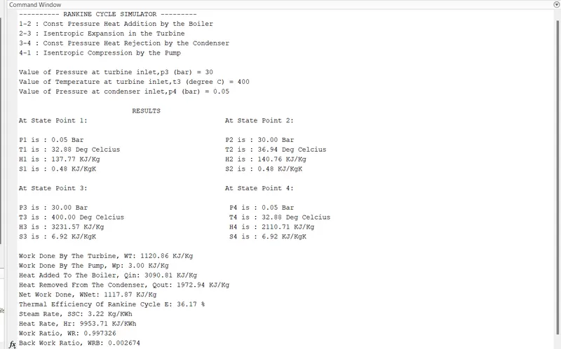
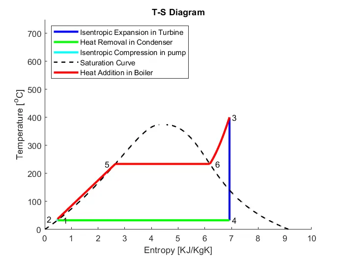
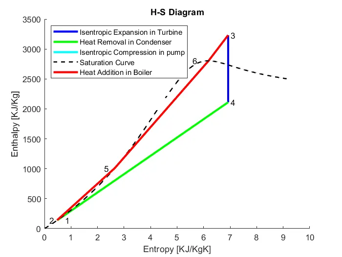
For User Defined Parameters

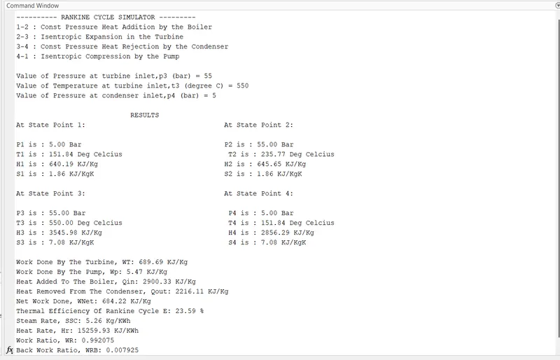
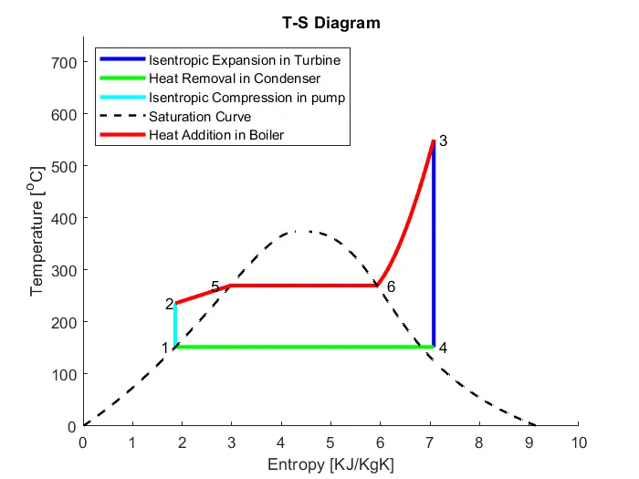
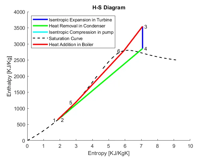
ERROR

Error Occured

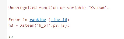
Step To Overcome Error: h3 = Xsteam('h_pT',p3,T3) changed to h3 = XSteam('h_pT',p3,T3)

Error Occured

Step To Overcome Error: plot(sat_sv,ts,'linewidth',1.5,'--','color','k') changed to plot(sat_sv,ts,'--','linewidth',1.5,'color','k')

Error Occured

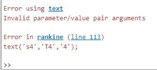
Step To Overcome Error: By refering to correct syntax text('s4','T4','4') changed to text(s4,T4,'4')

CONCLUSION

• Program to create a Rankine Cycle Simulator using MATLAB has been run successfully and calculated the state points based on user inputs.
• Ploted the corresponding T-s and h-s plots for the given set of inputs.

REFERENCE

Engineering Thermodynamics By P.K. Nag

Power Plant Engineering By P.K. Nag

Refrigeration & Air Conditioning By - R.S. Khurmi

https://in.mathworks.com/help/matlab/ref/input.html#:~:text=x%20%3D%20input(%20prompt%20)%20displays,input%20returns%20an%20empty%20matrix.

https://in.mathworks.com/matlabcentral/answers/250641-how-to-use-input-command

https://in.mathworks.com/help/matlab/ref/text.html

https://www.mathworks.com/help/matlab/ref/legend.html

https://www.mathworks.com/help/matlab/creating_plots/add-legend-to-graph.html