Week 4.1 - Genetic Algorithm

Genetic Algorithm

The genetic algorithm is a method for solving both constrained and unconstrained optimization problems that is based on natural selection, the process that drives biological evolution. The genetic algorithm repeatedly modifies a population of individual solutions. At each step, the genetic algorithm selects individuals from the current population to be parents and uses them to produce the children for the next generation. Over successive generations, the population "evolves" toward an optimal solution. You can apply the genetic algorithm to solve a variety of optimization problems that are not well suited for standard optimization algorithms

This flow chart outlines the main algorithmic steps.

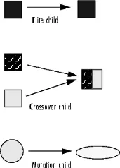
The genetic algorithm uses three main types of rules at each step to create the next generation from the current population:

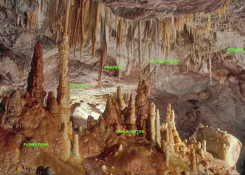
Stalagmite

A stalagmite is a type of rock formation that rises from the floor of a cave due to the accumulation of material deposited on the floor from ceiling drippings.

Syntax for Genetic Algorithm

x = ga(fun,nvars) finds a local unconstrained minimum, x, to the objective function, fun. nvars is the dimension (number of design variables) of fun.

x = ga(fun,nvars,A,b) finds a local minimum x to fun, subject to the linear inequalities A*x ≤ b. ga evaluates the matrix product A*x as if x is transposed (A*x').

x = ga(fun,nvars,A,b,Aeq,beq) finds a local minimum x to fun, subject to the linear equalities Aeq*x = beq and A*x ≤ b. (Set A=[] and b=[] if no linear inequalities exist.) ga evaluates the matrix product Aeq*x as if x is transposed (Aeq*x').

x = ga(fun,nvars,A,b,Aeq,beq,lb,ub) defines a set of lower and upper bounds on the design variables, x, so that a solution is found in the range lb ≤ x ≤ ub. (Set Aeq=[] and beq=[] if no linear equalities exist.)

x = ga(fun,nvars,A,b,Aeq,beq,lb,ub,nonlcon,options) minimizes with the default optimization parameters replaced by values in options. (Set nonlcon=[] if no nonlinear constraints exist.) Create options using optimoptions.

[x,fval] = ga(___), for any previous input arguments, also returns fval, the value of the fitness function at x.

Program to optimise the stalagmite function and find the global maxima of the function.

clear all
close all
clc

% inputs
x = linspace(0,0.5,200);
y = linspace(0,0.5,200);

% initialization
num_case = 50;

% creating 2D mesh
[xx , yy] = meshgrid(x,y);

for i = 1:length(xx)
    for j = 1:length(yy)
        input_vector(1) = xx(i,j);
        input_vector(2) = yy(i,j);
        f(i,j) = stalagmite_func(input_vector);
    end
end

figure('Name','surface plot')
surfc(xx,yy,-f)
shading interp
xlabel('x values')
ylabel('y values')
zlabel('z values')


% study 1 unbounded
tic

for i = 1: num_case
    [inputs,fval(i)] = ga(@stalagmite_func,2);
    xval(i) = inputs(1);
    yval(i) = inputs(2);
end

study_1 = toc;

% Ploting
figure('name',"Unbounded")
subplot(2,1,1)
surfc(xx,yy,-f)
xlabel('x values')
ylabel('y values')
title('case 1 (unbounded)','color','k')
shading interp
hold on
plot3(xval,yval,-fval,'Marker','o','markersize',5,'MarkerFaceColor','r')
subplot(2,1,2)
plot(-fval)
xlabel('no. of iteration')
ylabel('max function values')

% study 2 bounded
tic

for i = 1: num_case
    [inputs,fval(i)] = ga(@stalagmite_func,2,[],[],[],[],[0,0],[0.5,0.5]);
    xval(i) = inputs(1);
    yval(i) = inputs(2);
end

study_2 = toc;

% Plotting
figure('name','bounded')
subplot(2,1,1)
surfc(xx,yy,-f)
xlabel('x values')
ylabel('y values')
title('case 2 (bounded)','color','k')
shading interp
hold on
plot3(xval,yval,-fval,'Marker','o','markersize',5,'MarkerFaceColor','r')
subplot(2,1,2)
plot(-fval)
xlabel('no. of iteration')
ylabel('max function values')

% study 3 bounded with increase in population
options = optimoptions('ga');
options = optimoptions(options, 'populationsize',100);

tic

for i = 1: num_case
    [inputs,fval(i)] = ga(@stalagmite_func,2,[],[],[],[],[0,0],[0.5,0.5],[],options);
    xval(i) = inputs(1);
    yval(i) = inputs(2);
end

study_3 = toc;

% Plotting
figure('name','Bounded with increase in population')
subplot(2,1,1)
surfc(xx,yy,-f)
xlabel('x values')
ylabel('y values')
title('case 3 (bounded with increase in population)','color','k')
shading interp
hold on
plot3(xval,yval,-fval,'Marker','o','markersize',5,'MarkerFaceColor','r')
subplot(2,1,2)
plot(-fval)
xlabel('no. of iteration')
ylabel('max function values')

% study 4 bounded with more population size
options = optimoptions('ga');
options = optimoptions(options, 'populationsize',250);

tic

for i = 1: num_case
    [inputs,fval(i)] = ga(@stalagmite_func,2,[],[],[],[],[0,0],[0.5,0.5],[],options);
    xval(i) = inputs(1);
    yval(i) = inputs(2);
end

study_4 = toc;

% Plotting
figure('name','Bounded with more population size')
subplot(2,1,1)
surfc(xx,yy,-f)
xlabel('x values')
ylabel('y values')
title('case 4 (bounded with more population)','color','k')
shading interp
hold on
plot3(xval,yval,-fval,'Marker','o','markersize',5,'MarkerFaceColor','r')
subplot(2,1,2)
plot(-fval)
xlabel('no. of iteration')
ylabel('max function values')

% Display the x and y values
display(inputs)

Stalagmite Function Program

function [f] = stalagmite_func(input_vector)

% Inputs
x = input_vector(1);
y = input_vector(2);

% Function
f1x = (sin((5.1*pi).*x+0.5)).^6;
f1y = (sin((5.1*pi).*y+0.5)).^6;
f2x = exp((((x-0.0667).^2)/0.64).*(-4*log(2)));
f2y = exp((((y-0.0667).^2)/0.64).*(-4*log(2)));
fopt = f1x*f1y*f2x*f2y;
f = -fopt;

OUTPUT:

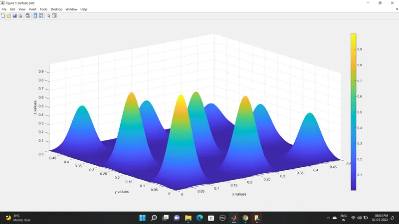
Stalagmite Function Surface Plot

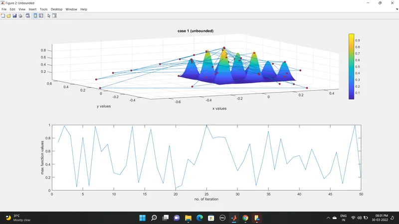
Case 1 : Unbounded

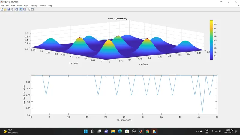
Case 2 : Bounded

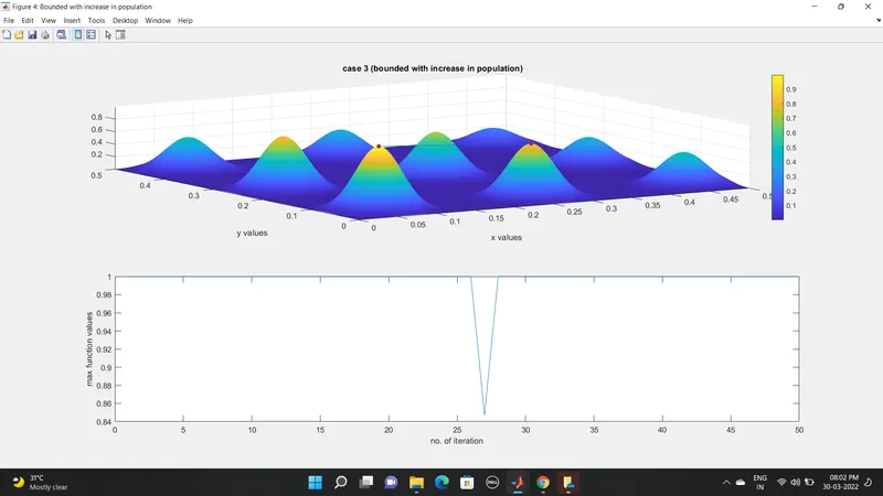
Case 3 : Bounded with increase in population

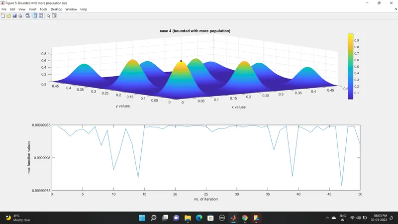
Case 4 : Bounded with more population

Explanation

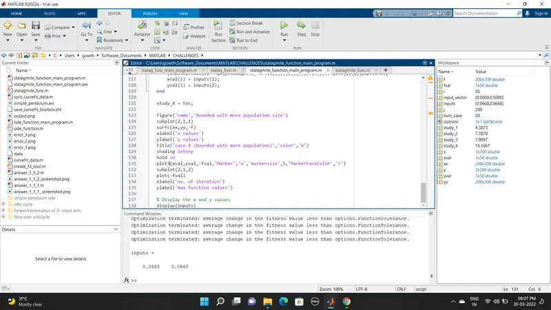
Create x and y values using linspace command then using mesh grid 2D array was obtained. A nested loop was created to assign the input values to the stalagmite function. A seperate program is written for stalagmite function. In the stalagmite function the minus(-) sign is given to find the least value in negative side while performing Genetic Algorithm. Normally Genetic Algorithm output is global minima. But we required global maxima. So, we again Put minus (-) sign to invert the answer(-fval). Tic - Toc command is used to get the running time of each case.

In the first case the boundary conditions are not defined and plots are made. In the figure both the surface plot and the graph for No. of iteration vs max function values are shown. Negative sign is given inside the surface function to get the stalagmite function upwards. In second case boundary condition is given. So, that the number of solution approches more accuracy and plotting is done. In case three and four the population is increases in the subsequent case to get more accruate result and plotting is done. By increasing the population size we get the global maxima. The x and y values for which the global maxima is found is displayed in the command window. Even we execute the program several times we get the same value as gobal maxima.

Mention the errors while programming.

Error 1:

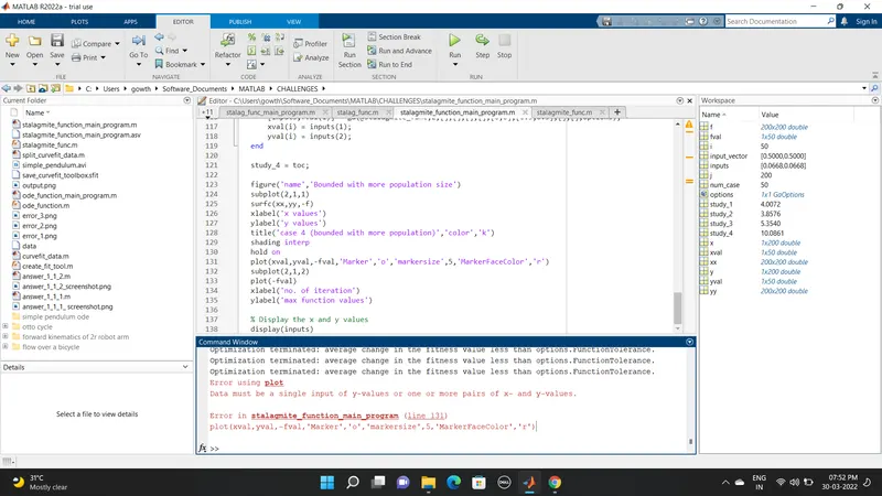
Solution 1: For three dimensional plot we have to use plot3 command. but i typed worngly as plot. So, after the error shown i changed my mistake.

Reference

1.Genetic Algorithm

2.stalagmites

3. GA Syntax