Project 2 - Rankine cycle Simulator

Rankine Cycle Simulator

AIM:

Create a Rankine Cycle Simulator using MATLAB.

OBJECTIVE:

1. Extracting steam and water properties from XSteam data.

1. To calculate all the state points of the Rankine Cycle based on user inputs.

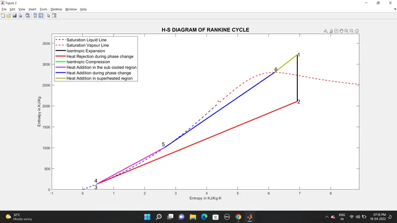
1. Plotting of Corresponding T-S Diagram and H-S Diagram for the given inputs.

THEORY:

The Rankine cycle is an idealized thermodynamic cycle describing the process by which certain heat engines, such as steam turbines or reciprocating steam engines, allow mechanical work to be extracted from a fluid as it moves between a heat source and heat sink. The Rankine cycle is named after William John Macquorn Rankine, a Scottish polymath professor at Glasgow University.

Heat energy is supplied to the system via a boiler where the working fluid (typically water) is converted to a high-pressure gaseous state (steam) in order to turn a turbine. After passing over the turbine the fluid is allowed to condense back into a liquid state as waste heat energy is rejected before being returned to boiler, completing the cycle. Friction losses throughout the system are often neglected for the purpose of simplifying calculations as such losses are usually much less significant than thermodynamic losses, especially in larger systems.

Four Important components of Rankine cycle

1. TURBINE

1. CONDENSER

1. PUMP

1. BOILER

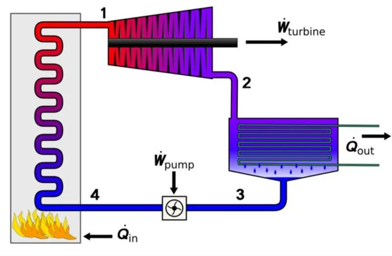
Four process of Rankine cycle

Process 1-2 Isentropic expansion

(Turbine 1-2): Superheated steam enters into the turbine and expands Isentropically resulting production of work. This result in decrease in temperature and pressure of vapour and some condensation occurs. The shaft of turbine connected to the generator. This results in the production of electricity. Mechanical energy is converted into work.

Work produces by turbine

wT = h1 – h2

Process 2-3 Constant pressure heat rejection

(Condenser 2-3): The expanded vapour from turbine is then passes through a condenser, where it condenses at a constant pressure and convert into liquid again. In the condenser the cooling water coil pass inside. Thus, heat transfer takes place. During condensation the heat is rejected

Heat rejection in condenser

QR = h2 – h3

Process 3-4 Isentropic compression

(Pump 3- 4): The water enters into the pump in saturated state. Then liquid is compressed isentropically unit it meets the boiler pressure.

Work done by the pump

wP = h3 – h4

Process 4-1 Constant pressure heat addition

(Boiler 4-1): The high-pressure water (compressed) from the pump enters into the boiler. The heat is added to the boiler to rese the temperature. So, that the water phase changes from liquid to superheated vapour state.

The heat is supplied in boiler

Qs = h1 – h4

The net work done by the system is

Wnet = wT - wP

Thermal efficiency of Rankine cycle is

η = (Net work done / Heat supplied) * 100

= (wT – wP )/ (h1 – h4)

Specific steam consumption

SSC = 3600/ Wnet

Back work ratio

Some of the power produced in the turbine of a gas turbine power plant is used to drive the pump

Back work ratio = wP / wT

PROGRAM

clear all
close all
clc

% Display the process
fprintf('\t\t\tRANKINE CYCLE SIMULATOR\n\n');
fprintf('PROCESS 1-2  ISENTROPIC EXPANSION IN TURBINE\n');
fprintf('PROCESS 2-3  CONSTANT PRESSURE HEAT REJECTION IN CONDENSER\n');
fprintf('PROCESS 3-4  ISENTROPIC COMPRESSION IN PUMP\n');
fprintf('PROCESS 4-1  CONSTANT PRESSURE HEAT ADDITION IN BOILER\n\n');

% Inputs
p1 = input('Enter the pressure at turbine inlet (in bar) :');
t1 = input('Enter the temperature at turbine inlet (in degree celcius) :');
p2 = input('Enter the pressure at condensor inlet (in bar) :');

% state point 1
s1 = XSteam('s_pt',p1,t1);
h1 = XSteam('h_pt',p1,t1);

% state point 2
s2 = s1;
sf2 = XSteam('sL_p',p2);
sg2 = XSteam('sV_p',p2);
hf2 = XSteam('hL_p',p2);
hg2 = XSteam('hV_p',p2);    % s2 = sf2 + x(sg2-sf2)

x = (s2-sf2)/(sg2-sf2);

if x<=1   % the point 2 in  liquid vapour mixture region or saturated vapour
    h2 = hf2 + x*(hg2 - hf2);
    t2 = XSteam('T_hs',h2,s2);
else
    Tsat_p2 = XSteam('Tsat_p',p2);
    t2 = XSteam('T_ps',p2,s2);
    cpV = XSteam('cp_pT',p2,t2);
    h2 = hf2 + cpV*(t2 - Tsat_p2);
end

% state point 3
t3 = t2;
p3 = p2;
s3 = XSteam('sL_p',p3);
h3 = XSteam('hL_p',p3);
v3 = XSteam('vL_p',p3);

% state point 4
p4 = p1;
s4 = s3;
t4 = XSteam('T_ps',p4,s4);
h4 = XSteam('h_ps',p4,s4);
v4 = XSteam('v_ps',p4,s4);

% state point 5
h5 = XSteam('hL_p',p1);
s5 = XSteam('sL_p',p1);
t5 = XSteam('T_ps',p1,s5);

% state point 6
t6 = t5;
h6 = XSteam('hV_p',p1);
s6 = XSteam('sV_p',p1);

% calculate the other output values
W_t = h1 - h2;                       % Work done by the turbine
W_p = h4 - h3;                       % Work done by the pump
W_net = W_t - W_p;             % Net work done by the system      
Q_in = h1 - h4;                      % Heat supplied
Q_out = h2 - h3;                     % Heat rejected
thermal_eff = (W_net / Q_in)*100;    % Thermal Efficiency

% steam rate (specific heat consumption)
s_s_c = (3600/ W_net);     

% Back work ratio
b_w_r = W_p/ W_t;

% Printing all state point values
fprintf('\n\t\t\tRESULTS\n');
fprintf('At State Point 1 \nP1 = %4.2f Bar\nT1 = %4.2f Degree Celcius\nH1 = %4.2f KJ/Kg\nS1 = %4.2f Kg/Kg-K\n\n',p1,t1,h1,s1)
fprintf('At State Point 2 \nP2 = %4.2f Bar\nT2 = %4.2f Degree Celcius\nH2 = %4.2f KJ/Kg\nS2 = %4.2f Kg/Kg-K\n\n',p2,t2,h2,s2)
fprintf('At State Point 3 \nP3 = %4.2f Bar\nT3 = %4.2f Degree Celcius\nH3 = %4.2f KJ/Kg\nS3 = %4.2f Kg/Kg-K\n\n',p3,t3,h3,s3)
fprintf('At State Point 4 \nP4 = %4.2f Bar\nT4 = %4.2f Degree Celcius\nH4 = %4.2f KJ/Kg\nS4 = %4.2f Kg/Kg-K\n\n',p4,t4,h4,s4)
fprintf('Calculation \nWork done by the turbine = %4.2f KJ/Kg\nWork done by the pump = %4.2f KJ/Kg\nNet work done by the system = %4.2f KJ/Kg\nHeat supplied to the system = %4.2f KJ/Kg\nHeat rejected in the system = %4.2f KJ/Kg\nThermal efficiency = %4.2f %%\nSpecific heat consumption = %4.2f KJ/Kwh\nBack work ratio = %4.6f\n\n',W_t,W_p,W_net,Q_in,Q_out,thermal_eff,s_s_c,b_w_r);

% Finding saturation temperature  corresponding entropy 
% for saturation line of T-S diagram
s_min =  0;
s_max = s1 + 2;
s = linspace(s_min,s_max,1000);
for j = 1 : length(s)
    tsat(j) = XSteam('Tsat_s',s(j));
end

% Finding critical temperature and critical pressure of water
c_temp_water = 373.946;      % degree celcius
c_pressure_water = 220.653;      % in bar
s_critical = XSteam('s_pT',c_pressure_water,c_temp_water);

% Finding saturation enthalpy using entropy and saturation pressure
% for saturation line on H-S Diagram
% liquid state saturation enthalpy before critical temperature
s_sat_L = linspace(s_min,s_critical,1000);
for k = 1 : length(s_sat_L)
    p_sat_L(k) = XSteam('psat_s',s_sat_L(k));
    h_sat_L(k) = XSteam('hL_p',p_sat_L(k));
end

% Gaseous state saturation enthalpy after critical temperature
s_sat_V = linspace(s_critical,s_max,1000);
for l = 1 : length(s_sat_V)
    p_sat_V(l) = XSteam('psat_s',s_sat_V(l));
    h_sat_V(l) = XSteam('hV_p',p_sat_V(l));
end

% To plot T-S Diagram
t_line = linspace(t5,t1,1000);
for i = 1 : length(t_line)
    s_line(i) = XSteam('s_pT',p1,t_line(i));
end

figure(1)
plot(s,tsat,'--','linewidth',1.5,'color','r')      % SATURATION LINE for T-S Diagram
hold on
plot([s1 s2],[t1 t2],'linewidth',2.5,'color','k')
hold on
plot([s2 s3],[t2 t3],'linewidth',2.5,'color','r')
hold on
plot([s3 s4],[t3 t4],'linewidth',2.5,'color','g')
hold on
plot([s4 s5],[t4 t5],'linewidth',2.5,'color','m')
hold on
plot([s5 s6],[t5 t6],'linewidth',2.5,'color','b')
hold on
plot([s6 s1],[t6 t1],'linewidth',2.5,'color',[0.7,0.7,0])
hold on
axis([0 s1+2 0 t1+100])
hold on
legend('Saturation Line','Isentropic Expansion','Heat Rejection during phase change','Isentropic Compression','Heat Addition in the sub cooled region','Heat Addition during phase change','Heat Addition in superheated region','location','northwest','fontsize',12);
xlabel('Entropy in KJ/Kg-K');
ylabel('Temperature in Degree Celcius');
title('T-S DIAGRAM OF RANKINE CYCLE','FontSize',15);
text(s1,t1,'1','FontSize',15)
text(s2,t2,'2','FontSize',15)
text(s3,t3,'3','FontSize',15,'HorizontalAlignment','right','VerticalAlignment','top')
text(s4,t4,'4','FontSize',15,'HorizontalAlignment','right','VerticalAlignment','bottom')
text(s5,t5,'5','FontSize',15,'HorizontalAlignment','right','VerticalAlignment','bottom')
text(s6,t6,'6','FontSize',15,'HorizontalAlignment','left')

% To plot H-S Diagram
figure(2)
plot(s_sat_L,h_sat_L,'--','linewidth',1.5,'color','b')      % SATURATION LIQUID LINE for H-S Diagram
hold on
plot(s_sat_V,h_sat_V,'--','linewidth',1.5,'color','r')      % SATURATION VAPOUR LINE for H-S Diagram
hold on
plot([s1 s2],[h1 h2],'linewidth',2.5,'color','k')
hold on
plot([s2 s3],[h2 h3],'linewidth',2.5,'color','r')
hold on
plot([s3 s4],[h3 h4],'linewidth',2.5,'color','g')
hold on
plot([s4 s5],[h4 h5],'linewidth',2.5,'color','m')
hold on
plot([s5 s6],[h5 h6],'linewidth',2.5,'color','b')
hold on
plot([s6 s1],[h6 h1],'linewidth',2.5,'color',[0.7,0.7,0])
hold on
axis([-1 s1+2 0 h1+500])
legend('Saturation Liquid Line','Saturation Vapour Line','Isentropic Expansion','Heat Rejection during phase change','Isentropic Compression','Heat Addition in the sub cooled region','Heat Addition during phase change','Heat Addition in superheated region','location','northwest','fontsize',12);
xlabel('Entropy in KJ/Kg-K');
ylabel('Enthalpy in KJ/Kg');
title('H-S DIAGRAM OF RANKINE CYCLE','FontSize',15);
text(s1,h1,'1','FontSize',15)
text(s2,h2,'2','FontSize',15)
text(s3,h3,'3','FontSize',15,'HorizontalAlignment','right','VerticalAlignment','top')
text(s4,h4,'4','FontSize',15,'HorizontalAlignment','right','VerticalAlignment','bottom')
text(s5,h5,'5','FontSize',15,'HorizontalAlignment','right','VerticalAlignment','bottom')
text(s6,h6,'6','FontSize',15,'HorizontalAlignment','left','VerticalAlignment','bottom')

OUTPUT:

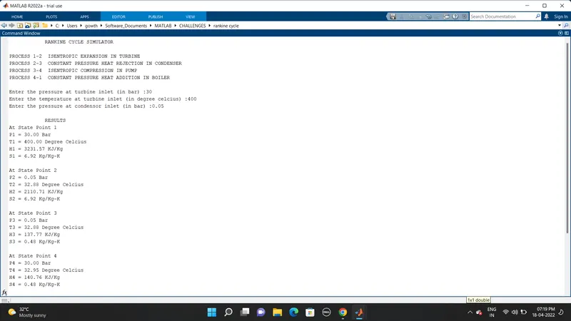
Command Window

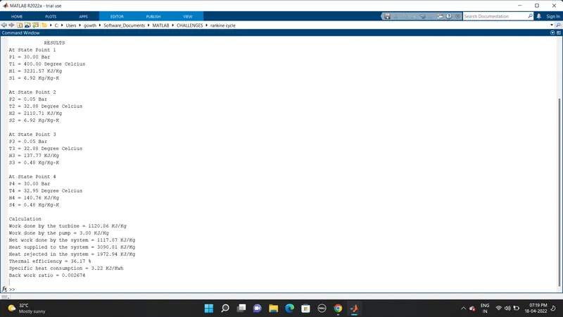
continue of command window

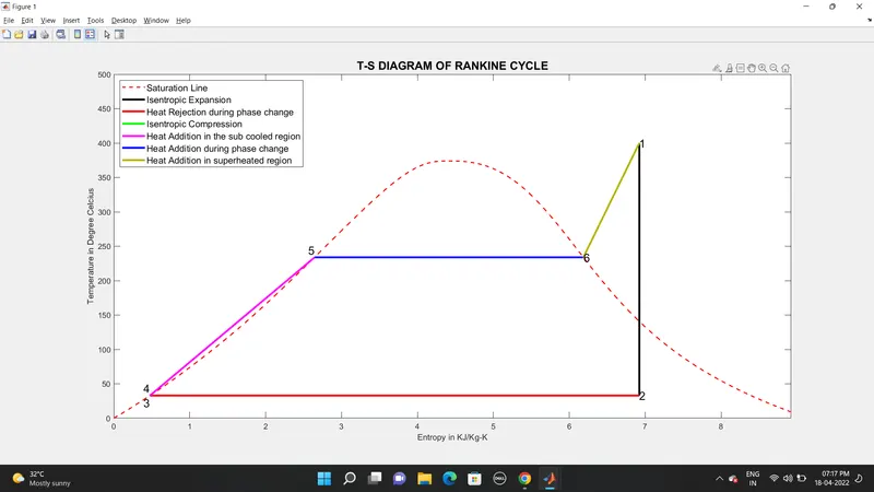
T-S Diagram

H-S Diagram

Step-wise explanation of your code

• First display the process of the Rankine cycle simulator
• Then using the ‘input’ command, the operating pressure of boiler, condenser and turbine inlet temperature are taken as input from the user.
• In State point 1 the values of entropy and enthalpy are determined from the xsteam library using p1 as input.
• In state point 2 using the entropy relation calculate the value of enthalpy and temperature using the xsteam library p2 and s2 as input.
• In state point 3 the temperature and pressure are same as in state point 2 (p3 = p2; t3 = t2) using this relation determine the entropy, enthalpy and volume from xsteam library
• In state point 4 using the relation p4 = p1 and s4 = s3. Determine the temperature, enthalpy and volume using the xsteam library.
• Determine the entropy, enthalpy and temperatures for state point 5 & 6 for plotting T-S Diagram & H-S Diagram.
• Now calculate

1. the work done by turbine
2. work done by the pump
3. Net work done by the system
4. Heat supplied in the boiler
5. Heat rejected in the condenser
6. Thermal efficiency
7. Specific heat consumption
8. Back work ratio

• Print all the state point values and the above calculated details in the command window using ‘fprintf’ command.
• For plotting saturation line in the T-S Diagram find the saturation temperatures for corresponding entropy using a for loop
• Using the critical pressure and temperature of water data find the entropy by using xsteam library. Determine the saturation liquid temperature and saturation vapour temperature using the entropy
• Plotting is done for both T-S & H-S Diagram using the plot commands. Annotations are assigned using text command.
• Labelling the plots and give the title with legends. For both T-S & H-S Diagram
• Then using text command give the process number for easy understanding.

Mention the errors faced while programming.

Error 1 :

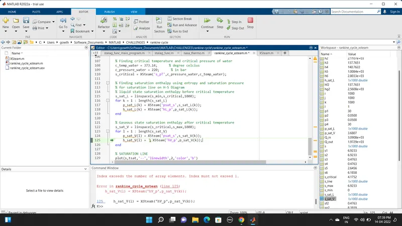
Solution 1 :

While using foe loop for gaseous state saturation enthalpy. Instead of using the 'l' for geting the iteration value, I type as 'K'. After error shown i corrected my mistake.

Reference:

Specific Steam Consumption

Rankine_cycle

Water critical-pressure & critical-temperature