Week 4.1 - Genetic Algorithm
AIM :
- To Write a code in MATLAB to optimise the stalagmite function and find the global maxima of the function.
- To expalin the concept of genetic algorithm and explain the syntax for ga in MATLAB.
- To Plot graphs for all 3 studies and for F maximum vs no. of iterations.
THEORY :
GENETIC ALGORITHM : The genetic algorithm is a method for solving both constrained and unconstrained optimization problems that is based on natural selection, the process that drives biological evolution. The genetic algorithm repeatedly modifies a population of individual solutions. At each step, the genetic algorithm selects individuals from the current population to be parents and uses them to produce the children for the next generation. Over successive generations, the population "evolves" toward an optimal solution. You can apply the genetic algorithm to solve a variety of optimization problems that are not well suited for standard optimization algorithms, including problems in which the objective function is discontinuous, nondifferentiable, stochastic, or highly nonlinear. The genetic algorithm can address problems of mixed integer programming, where some components are restricted to be integer-valued.
This flow chart outlines the main algorithmic steps :

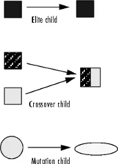
The genetic algorithm uses three main types of rules at each step to create the next generation from the current population:
-
Selection rules select the individuals, called parents, that contribute to the population at the next generation. The selection is generally stochastic, and can depend on the individuals' scores.
-
Crossover rules combine two parents to form children for the next generation.
-
Mutation rules apply random changes to individual parents to form children.
WORKING OF GENETIC ALGORITHM :
The working of genetic algorithm is as follows,
-
The algorithm begins by creating a random initial population.
-
-
Scores each member of the current population by computing its fitness value. These values are called the raw fitness scores.
-
Scales the raw fitness scores to convert them into a more usable range of values. These scaled values are called expectation values.
-
Selects members, called parents, based on their expectation.
-
Some of the individuals in the current population that have lower fitness are chosen as elite. These elite individuals are passed to the next population.
-
Produces children from the parents. Children are produced either by making random changes to a single parent—mutation—or by combining the vector entries of a pair of parents—crossover.
-
Replaces the current population with the children to form the next generation.
Syntax for GA:
x= ga(finds a local unconstrained minimum,fun,nvars)x, to the objective function,fun.nvarsis the dimension (number of design variables) offun.x= ga(fun,nvars,A,b,Aeq,beq,lb,ub)x, so that a solution is found in the rangelb≤x≤ub. (SetAeq=[]andbeq=[]if no linear equalities exist.)x= ga(fun,nvars,A,b,Aeq,beq,lb,ub,nonlcon,options)options. (Setnonlcon=[]if no nonlinear constraints exist.) Createoptionsusingoptimoptions -
CODE EXPLANATION : Coding and minimizing the fitness function using genetic algorithm.
STEP 1 :FITNESS FUNCTION CODE
A fitness function must take one input x and input y where x and y is a row vector with as many elements as number of variables in the problem. The fitness function computes the value of the function and returns that scalar value in its one return argument f.
function[f]= stalagmite(input_vector)
% inputs
x=input_vector(1);
y=input_vector(2);

% defining the term
term1=(sin((5.1*pi*x)+0.5))^6 ;
term2=exp((-4)*log(2)*((x-0.0667)^2)/0.64);
term3=(sin((5.1*pi*y)+0.5))^6 ;
term4=exp((-4)*log(2)*((y-0.0667)^2)/0.64);

 f=-(term1*term2*term3*term4);
end
STEP 2: MINIMIZE USING GA:
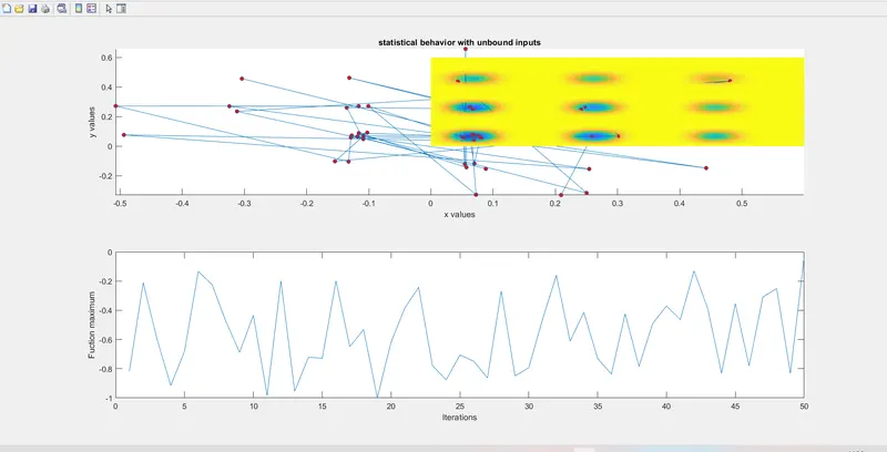
STUDY 1 statistical behavior shows the minimization using the ga
To minimize the fitness function using ga pass a function handle to the fitness function as well as the number of variables in the problem .x = ga(fun,nvars)x, to the objective function, fun. nvars is the dimension (number of design variables) of fun. here fun is defined as stalagmite and nvars as 2.
%study 1--statistical behavior
tic
for i=1:num_cases
    [inputs,fopt(i)]=ga(@stalagmite,2);
    xopt(i)=inputs(1);
    yopt(i)=inputs(2);
end
study_time1=toc
%plotting
figure(1)
subplot(2,1,1) % used to plot multiple plots on same figure
hold on
surfc(x,y,f)    %  creates a three-dimensional surface plot with a contour plot underneath
shading interp    % varies the color in each line segment and face by interpolating the colormap index or true color value across the line or face
xlabel('x values')
ylabel('y values')
title('statistical behavior with unbound inputs')
plot3(xopt,yopt,fopt,'marker','o','markersize',5,'MarkerFaceColor','r') %plots coordinates in 3-D space
subplot(2,1,2)
plot(fopt)
xlabel('Iterations')
ylabel('Fuction maximum')
STEP 3:MINIMIZING USING THE ADDITIONAL PARAMETER:
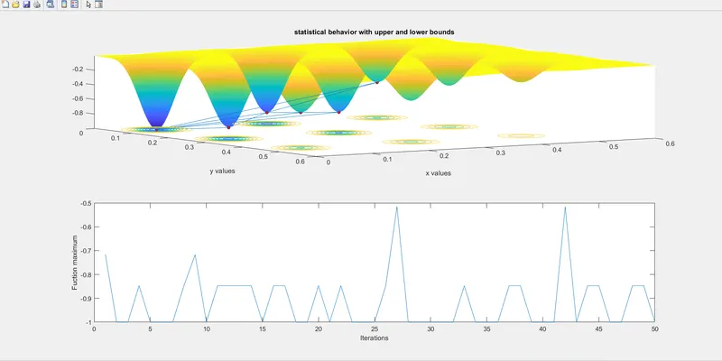
STUDY 2 statistical behavior with upper and lower bounds represents minimizing using the additional parameters.To minimize the fitness function using ga , pass a function handle to the fitness function as well as the number of variables in the problem. To have ga examine the relevant region, include bounds lower bound as [0 0] and the upper bounds[1 1] Pass the bounds as the fifth and sixth arguments after numberofvariable.
x = ga(fun,nvars,A,b,Aeq,beq,lb,ub)lb ≤ x ≤ ub. (Set Aeq=[] and beq=[] if no linear equalities exist.)
% study 2-- statistical behavior with upper and lower bounds
tic
for i=1:num_cases
    [inputs,fopt(i)]=ga(@stalagmite,2,[],[],[],[],[0;0],[1;1]);
    xopt(i)=inputs(1);
    yopt(i)=inputs(2);
end
study_time2=toc
figure(2)
subplot(2,1,1)
hold on
surfc(x,y,f)
shading interp
xlabel('x values')
ylabel('y values')
title('statistical behavior with upper and lower bounds')
plot3(xopt,yopt,fopt,'marker','o','markersize',5,'MarkerFaceColor','r')
subplot(2,1,2)
plot(fopt)
xlabel('Iterations')
ylabel('Fuction maximum')
STEP 3: SPECIFY POPULATION OPTION:
Population options can have a large effect on solver performance. The speed of each iteration depends on the population size: a larger population leads to slower iterations. Conversely, a larger population leads to ga exploring more thoroughly, so can lead to a better solution. Similarly, a wider initial range can lead to more thorough exploration, but can require a larger population to explore the wider range with a similar thoroughness.
Specify Population Size
ga creates a default initial population by using a uniform random number generator. The default population size used by ga is 50 when the number of decision variables is less than 5, and 200 otherwise. The default size might not work well for some problems; for example, a smaller population size can be sufficient for smaller problems. Since the current problem has only two variables, specify a population size of 220. Set the value of the option populationsize to 220 in the existing options,opts.
Modify the value of the option polulationsize in the existing options,opts.
opts.populationsize = [220];
Run the ga solver.
[x,Fval,exitFlag,Output] = ga(FitnessFunction,numberOfVariables,[],[],[], ...
    [],[],[],[],opts);

optimoptions syntax:
% study 3--statistical behavior with increasing the iteration of Ga
options=optimoptions('ga')
options=optimoptions(options,'PopulationSize',220);
tic
for i=1:num_cases
    [inputs,fopt(i)]=ga(@stalagmite,2,[],[],[],[],[0;0],[1;1],[],[],options);
    xopt(i)=inputs(1);
    yopt(i)=inputs(2);
end
study_time3=toc
figure(3)
subplot(2,1,1)
hold on
surfc(x,y,f)
shading interp
xlabel('x values')
ylabel('y values')
title('statistical behavior with increasing iteration GA')
plot3(xopt,yopt,fopt,'marker','o','markersize',5,'MarkerFaceColor','r')
subplot(2,1,2)
plot(fopt)
xlabel('Iterations')
ylabel('Fuction maximum')
STEP 4:
Reproduce Results
By default,ga starts with a random initial population created using MATLAB random number generators. The solver produces the next generation using ga operators that also use these same random number generators. Every time a random number is generated, the state of the random number generators changes. So, even if you do not change any options, you can get different results when you run the solver again.
Reset the stream and rerun ga . The results are identical to the previous run.as rng(thestate).
STEP 5:
CONCULSION :The best function value can improve or get worse based on the specified operators. Experimenting with different operators is often the best way to determine which set of operators works best for your problem.
MATLAB CODE :
MAIN CODE
clear
close all
clc
x=linspace(0,0.6,150);
y=linspace(0,0.6,150);

% creating 2-D mesh
[xx,yy]=meshgrid(x,y);

num_cases=50;


for i=1:length(xx)
    for j=1:length(yy)
        input_vector(1)=xx(i,j);
        input_vector(2)=yy(i,j);
f(i,j)=stalagmite(input_vector);
    end
end

%study 1--statistical behavior
tic
for i=1:num_cases

    [inputs,fopt(i)]=ga(@stalagmite,2);
    xopt(i)=inputs(1);
    yopt(i)=inputs(2);
end
study_time1=toc
%plotting
figure(1)
subplot(2,1,1) % used to plot multiple plots on same figure
hold on
surfc(x,y,f)    %  creates a three-dimensional surface plot with a contour plot underneath
shading interp    % varies the color in each line segment and face by interpolating the colormap index or true color value across the line or face
xlabel('x values')
ylabel('y values')
title('statistical behavior with unbound inputs')
plot3(xopt,yopt,fopt,'marker','o','markersize',5,'MarkerFaceColor','r') %plots coordinates in 3-D space
subplot(2,1,2)
plot(fopt)
xlabel('Iterations')
ylabel('Fuction maximum')

% study 2-- statistical behavior with upper and lower bounds
tic
for i=1:num_cases
    [inputs,fopt(i)]=ga(@stalagmite,2,[],[],[],[],[0;0],[1;1]);
    xopt(i)=inputs(1);
    yopt(i)=inputs(2);
end
study_time2=toc
figure(2)
subplot(2,1,1)
hold on
surfc(x,y,f)
shading interp
xlabel('x values')
ylabel('y values')
title('statistical behavior with upper and lower bounds')
plot3(xopt,yopt,fopt,'marker','o','markersize',5,'MarkerFaceColor','r')
subplot(2,1,2)
plot(fopt)
xlabel('Iterations')
ylabel('Fuction maximum')

% study 3--statistical behavior with increasing the iteration of Ga
options=optimoptions('ga')
options=optimoptions(options,'PopulationSize',220);
tic
for i=1:num_cases
    rng(thestate);
    [inputs,fopt(i)]=ga(@stalagmite,2,[],[],[],[],[0;0],[1;1],[],[],options);
    xopt(i)=inputs(1);
    yopt(i)=inputs(2);
end
study_time3=toc
figure(3)
subplot(2,1,1)
hold on
RESULT/OUTPUT :
1. plot for the study 1 statistical behavior with nobounds
2. Plot for the study 2 statistical behavior with upper and lower bounds.
3.Plot for study 3 statistical behavior increasing the population size to get the maximum point.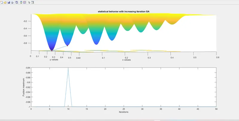
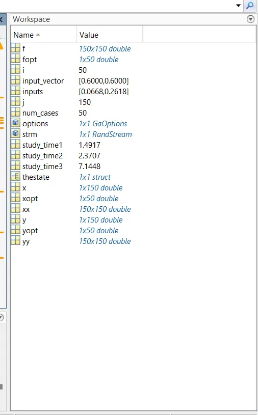
4.Result showing the time study.
REFERENCE :https://www.mathworks.com/help/matlab/