Project 2 - Rankine cycle Simulator
AIM : To Create a Rankine Cycle Simulator using MATLAB.
OBJECTIVE :
- To calculate the state points of the Rankine Cycle based on given inputs.
- To plot the corresponding T-s and h-s plots for the given set of inputs.
- To Calculate the Thermal Efficiency of the Rankien Cycle and Steam Rate.
THEORY : RANKINE CYCLE
Simple Rankien cycle Consists of the following reversible processes.
1.Isentropic Expansion`(1rarr2)` of steam in turbine.
2.Isobaric Cooling `(2rarr3)` of steam in condenser.
3.Isentropic Pumping `(3rarr4)` of saturated liquid (water) to boiler.
4.Isobaric Heating `(4rarr1)` in boiler.
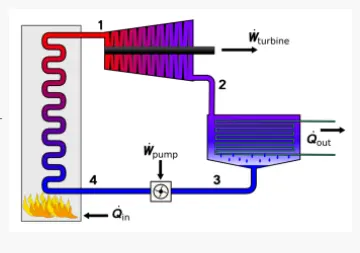
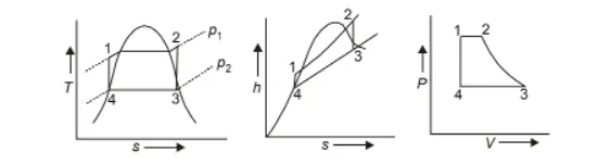
fig: Simple Rankien Cycle and T-S ,H-S and P-V Diagram is as shown in above fig.
1.Cycle Efficiency :Applying the steady flow energy equation to each of the processes on the basis of unit mass of working substance and neglecting changes in kinetic energy and potential energy , the heat supplied and heat rejected is given as,
`Q_s=h_1-h_4`
`Q_R=h_2-h_3`
work done by the system on the turbine , and the work done by the pump on the steam respectively,are
`W_t=h_2-h_1`
`W_p=h_4-h_3`
Therefore, the efficiency of rankien cycle is
`eta_(Rankien)=(W_(Net))/(Q_s)`
`=(Wt-Wp)/Q_s`
`=((h_1-h_2)-(h_4-h_3))/((h_1-h_4))`
`=1-(h_2-h_3)/(h_1-h_4)`
2.Pump Work :Considering the water as incompressive fluid, the work done by the pump on water during isentropic process (`3rarr4,d_s=0`)can be found using,
`T_(ds)=dh-vdp`
`dh=vdp`
since the change in specific volume is negligible,
`Deltah=vDeltap`
Hence,
`W_p=h_4-h_3=v_3(p_1-p_2)`
3.Steam Rate :Thecapacity of steam power plant is generally expressed in terms of steam rate(kg/h-kW),which is defined as the rate of steam flow required to produce unit shaft output power.
Steam rate =`3600/(W_t-W_p)`kg/h.
MATLAB CODE :
clear
close all
clc
% Rankien cycle simulator
fprintf('Rankien Cycle Simulator\n')

% displaying the Rankien cycle processes
fprintf('1-2 is Isentropic Expansion in the Turbine\n')
fprintf('2-3 is Constant Pressure Heat Rejection by the Condensor\n')
fprintf('3-4 is Isentropic Compression in the Pump\n')
fprintf('4-1 is Constant Pressure Heat Addition by the Boiler\n')

% defining the given inputs P1,T1,P2
p1=input('Enter the pressure at the Turbine Inlet (in Bar):');
t1=input('Enter the Temperature at the Turbine Inlet (in Degree Celcius):');
p2=input('Enter the pressure at Condenser (in Bar):');

% extracting the Enthalpy & Entropy from the XSteam Table
h1=XSteam('h_pT',p1,t1); % entalhpy for pressure & temperature for super heated steam
s1=XSteam('s_pT',p1,t1); % entropy for pressure & temperature for super heated steam

% for process 1-2 reverible adiabatic process
%entropy is constant
s2=s1;
sf2=XSteam('sL_P',p2);
sg2=XSteam('sV_P',p2);
hf2=XSteam('hL_P',p2);
hg2=XSteam('hV_P',p2);
hfg2=hg2-hf2;
sfg2=sg2-sf2;
x2=((s2-sf2)/(sfg2)); % X2 is the Dryness Fraction
h2=hf2+(x2.*(hfg2));

% at state point 3
% pressure is constant
p3=p2;
h3=XSteam('hL_P',p3);
s3=XSteam('sL_P',p3);
v3=XSteam('vL_P',p3);

% Entropy is constant
s4=s3;
p4=p1;

% Pump work Wp=h4-h3=v3(p1-p2)
Wp=v3*(p1-p2)*100;
h4=Wp+h3;

% work done by the steam on the turbine
WT=h1-h2;

% net work done (expansion work-pump work)
Wnet=(WT-Wp);

% heat supplied
Q1=h1-h4;

% Efficiency of Rankien cycle
efficiency=(Wnet/Q1)*100;

%Steam rate in Kg/h
steam_rate=(3600/(WT-Wp));

% At state point 3 finding temperature to plot the points
t3=XSteam('Tsat_P',p3);
t2=t3;
Cp4=XSteam('Cp_ps',p4,s4);
Cv4=XSteam('Cv_ps',p4,s4);
k=Cp4/Cv4;
t4=t3/((p3/p4)^((k-1)/k));

%calculating temperature ,enthalpy,entropy at liquid and vapor
t6=XSteam('Tsat_p',p1);
s5=XSteam('sL_p',p1);
s6=XSteam('sV_p',p1);
h5=XSteam('hL_p',p1);
h6=XSteam('hV_p',p1);
t5=t6;

%plotting
T=linspace(1,400,1000);
for i=1:length(T)
    sf(i)=XSteam('sL_T',T(i));
    sg(i)=XSteam('sV_T',T(i));
    hf(i)=XSteam('hL_T',T(i));
    hg(i)=XSteam('hV_T',T(i));
end
% plotting T-s diagram
figure(1)
hold on
plot(sf,T,'color','r','linewidth',2)
plot(sg,T,'color','r','linewidth',2)
plot([s1 s2],[t1 t2],'color','b','linewidth',1.5)
plot([s2 s3],[t2 t3],'color','b','linewidth',1.5)
plot([s3 s4],[t3 t4],'color','b','linewidth',1.5)
plot([s4 s5],[t4 t5],'color','b','linewidth',1.5)
plot([s5 s6],[t5 t6],'color','b','linewidth',1.5)
sc1=linspace(s6,s1,1000);
for l=1:length(sc1)
    Tc1(l)=XSteam('T_ps',p1,sc1(l));
end
plot(sc1,Tc1,'color','b','linewidth',1.5)
text(s1-0.1,t1+12,'1','fontsize',10)
text(s2,t2-5,'2','fontsize',10)
text(s3,t3,'3','horizontalalignment','right','verticalalignment','top','fontsize',10)
text(s4,t4,'4','horizontalalignment','right','verticalalignment','bottom','fontsize',10)
xlabel('Enthalpy [kJ/kg]','fontsize',14)
ylabel('Temperature [Degree celcius]','fontsize',14)
title('T-S Diagram For Rankien Cycle','fontsize',12)

% plotting the H-S  diagram
figure(2)
hold on
plot(sf,hf,'color','r','linewidth',2)
plot(sg,hg,'color','r','linewidth',2)
plot([s1 s2],[h1 h2],'color','b','linewidth',1.5)
plot([s2 s3],[h2 h3],'color','b','linewidth',1.5)
plot([s3 s4],[h3 h4],'color','b','linewidth',1.5)
plot([s4 s5],[h4 h5],'color','b','linewidth',1.5)
plot([s5 s6],[h5 h6],'color','b','linewidth',1.5)
sc2=linspace(s6,s1,1000);
for k=1:length(sc2)
    hc1(k)=XSteam('h_ps',p1,sc2(k));
end
plot(sc2,hc1,'color','b','linewidth',1.5)
text(s1,h1+50,'1','fontsize',10)
text(s2,h2-50,'2','fontsize',10)
text(s3,h3,'3','horizontalalignment','right','verticalalignment','top','fontsize',10)
text(s4,h4,'4','horizontalalignment','right','verticalalignment','bottom','fontsize',10)
xlabel('Entropy [kJ/kgK]','fontsize',14)
ylabel('Enthalpy [kJ/kg]','fontsize',14)
title('H-S Diagram For Rankien Cycle','fontsize',12)

% displaying the Result in command window
fprintf('RESULTS\n')
fprintf('At State Point 1:\nP1 is : %5.3f Bar\nT1 is : %5.3f Degree Celcius\nH1 is : %5.3f kJ/kg\nS1 is : %5.3f kJ/kgK\n',p1,t1,h1,s1)
fprintf('At State Point 2:\nP2 is : %5.3f Bar\nT2 is : %5.3f Degree Celcius\nH2 is : %5.3f kJ/kg\nS2 is : %5.3f kJ/kgK\n',p2,t2,h2,s2)
fprintf('X2 is : %5.3f\n',x2)
fprintf('At State Point 3:\nP3 is : %5.3f Bar\nT3 is : %5.3f Degree Celcius\nH3 is : %5.3f kJ/kg\nS3 is : %5.3f kJ/kgK\n',p3,t3,h3,s3)
fprintf('At State Point 4:\nP4 is : %5.3f Bar\nT4 is : %5.3f Degree Celcius\nH4 is : %5.3f kJ/kg\nS4 is : %5.3f kJ/kgK\n\n',p4,t4,h4,s4)
fprintf('Work Done By Turbine (Wt) is : %5.3f kJ/kg\n',WT)
fprintf('Work Done By Pump (Wp) is : %5.3f kJ/kg\n',Wp)
fprintf('Net Work Done By (Wnet) is : %5.3f kJ/kg\n',Wnet)
fprintf('Thermal Efficiency is : %5.3f percent\n',efficiency)
fprintf('Steam Rate is : %5.3f kg/h\n',steam_rate)
CODE EXPLANATION :
STEP 1:
- Start the MATLAB program with clear removes all variables from the current workspace, releasing them from system memory.close all closes the one or more figure window.clc clears the command window.
- fprintf Write data to text file to print the Rankien Cycle Simulator in the output window.
- Displaying the Rankien cycle processes using the fprintf command to display all the following process as mention in the above theory.
- Defining the given inputs P1,T1,P2
T1=Turbine Inlet temperature = 400° C
P1=Turbine Inlet Pressure = 30 bars
P2=Turbine Outlet Pressure = 0.05 bars = Condenser Inlet Pressure.
STEP 2 :
Extracting the Entropy and Enthalpy from the XSteam table for pressure & temperature for super heated steam
X.- The state points of the Rankine Cycle based on given inputs is calculated.
- The plot for corresponding T-s and h-s is ploted for the given set of inputs.
- The Thermal Efficiency of the Rankien Cycle and Steam Rate is calculated.
COMMAND WINDOW :
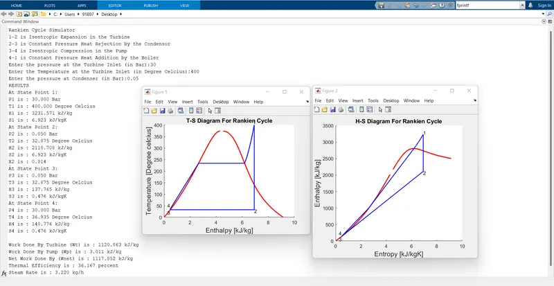
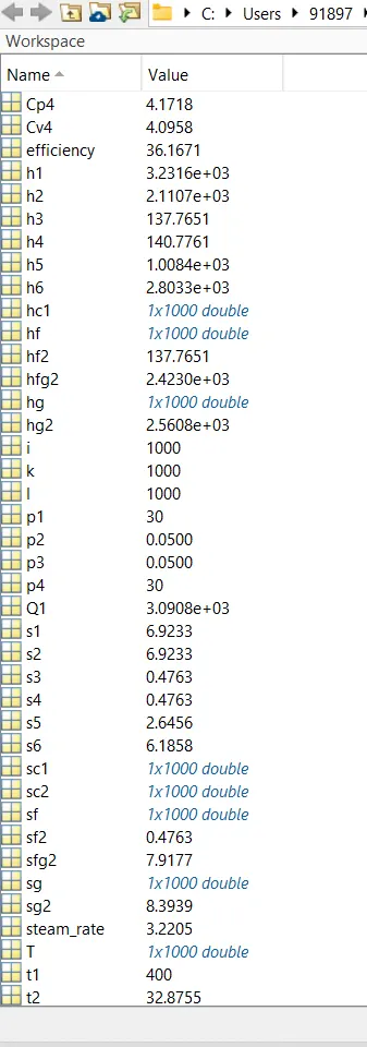
WORKSPACE MEMORY : The workspace memory is as shown in below figure which gives the values of the state points enthalpy ,entropy all the values is stored in workspace memory.
(a) By reducing heat addition in boiler, which could be realized by preheating water entering into it.
(b) By increasing steam turbine expansion work, i.e. by increasing expansion ratio within limiting dryness fraction considerations.
(c) By reducing feed pump work.
(d) By using heat rejected in condenser for feed water heating. etc.