Matlab program to solve otto cycle

AIM : To Write a Matlab code to solve an otto cycle with following requirement

• The code should create a PV diagram
• calculating the thermal efficiency of the engine.

THEORY :

Air standard Otto cycle is used for the SI Engines (Spark Ignition Engine). The cycle Contains Mainly four Processes. In the overall cycle, suction and Exhaust are neglected, also power consumption is not considered.
The Ideal Otto cycle consists of the four processes which are as below.

1–2 Reversible Adiabatic compression (Or) Isentropic Compression.
2–3 Constant Volume Heat Addition.
3–4 Reversible Adiabatic Expansion (Or) Isentropic Expansion.
4–1 Constant Volume Heat Rejection.

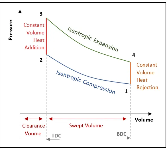
figure shows the Ideal PV Diagram

Terms in the Otto cycle:
As we know the basic otto cycle from above, there are two terms in induced TDC and BDC. Where TDC is called Top dead Centre which is Extreme position of the piston at the top end of cylinder similarly BDC is Extreme position at the bottom end of the cylinder.

i. Compression ratio (cr):- It is the ratio of volume before compression to the volume after compression.

Compression ratio (cr) = Volume before compression/volume after compression

also, Compression ratio (cr) = `(Vs+Vc)/(Vc)`

Where:-

V1= volume before compression = V_swept + V_clearance

V2 = volume after compression = V_clearance

Vs = V_swept , Vc = V_clearance

Therefore, Compression ratio (cr) = `(V1)/(V2)`

ii. Expansion ratio (er):- It is the ratio of volume after Expansion to the volume before compression.

Similarly, as the compression ratio, we can get an Expansion ratio.

Therefore, Expansion ratio (er) = `(V4)/(V3)`

Note:- for Otto cycle compression Ratio = Expansion ratio i.e (cr=er).

iii. Swept volume and Clearance volume:- Swept Volume (V_s) is a volume Before compression stroke. Also known as stoke volume and Displacement volume. Similarly, Clearance volume (V_c) is a volume after compression stroke.

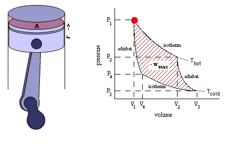
The Behavior of the piston and crank cause changes in the process of the Otto cycle PV diagram is as shown below.

DEFINING STATE VARIABLES:

State variable at Point-1:

i. Initial Pressure & Temperature:

P1= 101325 pa, T1= 500 K

ii. Engine Geometry parameters:

Bore (D) = 0.1 m

Stroke (L) = 0.1 m

Connceting rod Length (con_rod) = 0.15 m

And Compression Ratio (cr) = 12

iii. Swept volume and Clearance volume:

Clearance volume `V_c = V_s/(cr-1)`

Swept Volume `V_s = (pi/4)*D²*L`

Where:-
cr = compression ratio, D = Bore and L = Stroke

State Variable at point-2:

i. Calculating Pressure at point 2 (P2):

Due to isentropic compression, we can apply the PV Relation here.

P1V1^`gamma` = P2V2^`gamma`

Where, P2 is Unkown to us which can be calculated with the help of the relation between the volume, pressure and compression ratio

Also, we can calculate the P2 as follow

Cr = V1/V2 = (P2/P1)^`gamma`

Therefore, `P2 = P1 * ( cr )^`gamma``

ii. Calculating temp at point 2 (T2):

To get the value of temp T2 we are using the ideal gas equation as follows.

P1V1 = mRT1 , mR = P1V1/T1

P2V2 =mRT2 , mR = P2V2/T2

Therefore, P1V1/T1 = P2V2/T2

Hence, `T2 = P2*V2*(T1)/(P1*V1)`

State Variable at point-3:

i. Calculating Volume at point 3 (V3):

`V3=V2`

ii. Calculating Pressure at point 3 (P3):

By using the ideal gas equation

`P3 = P2 * (T3)/(T2)`

State Variable at point-4:

i. Calculating Volume at point 4 (V4):

`V1= V4`

ii. Calculating Pressure at point 3 (P3):

Also from P3V3^gamma = P4V4^gamma

`P4 = P3 *((V3)/(V4))^gamma`

EXPLANATION OF CODE :

Using the clear all removes all variables from the current workspace

close all closes the one or more figure window

clc clears all the command window

declaring the input variables

initiating the state variables at state 1 as the P1 and T1 are known

defining the engine geometric parameters

calculating the Swept volume and Clearance volume using the above formulae

calculating the value of T2 and P2 at state variable at state point 2
using the equation P2V2^gamma =P1V1^gamma and T2 = P2*V2*T1/(P1*V1)

P1*V1^gamma taking as constant for defining the volume compression

defining the function to Declare function name, inputs, and outputs for V_compression =engine_kinematics(bore,stroke,con_rod,cr,180,0) inside this function the array of crank angle was introduced and volume values at each angle was calculated.

similarly calculating the state variable at state point 3 and state point 4 for expansion process

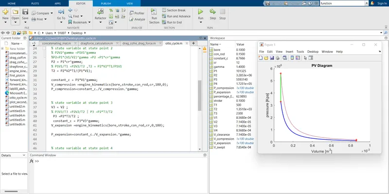
using the plot command we get a PV diagram having four points in it which represent state points

Calculating the Thermal Efficiency of the otto cycle ,

percentage_Efficiency = `1-(cr^(gamma-1))^-1*100`.

Plotting the graph pressure vs volume

MATLAB CODE :

clear all
close all
clc
%input 
gamma = 1.4;
T3 =2300 ;

% state variable state point 1
P1 = 101325 ;
T1 = 500 ;

% engine geometric parameter
bore = 0.1 ;
stroke = 0.1 ;
con_rod = 0.15 ;
cr = 12 ;

% calculating swept volume and the clearance volume
V_swept = pi/4*bore^2*stroke;
V_clearance = V_swept/(cr-1);
V1 = V_swept+V_clearance;
V2 = V_clearance;

% state variable at state point 2
% P2V2^gamma =P1V1^gamma
%P2=P1*(V1/V2)^gamma =P2 =P1*cr^gamma
P2 = P1*cr^gamma;
% P1V1/T1 =P2V2/T2 ,T2 = P2*V2*T1/P1V1
T2 = P2*V2*T1/(P1*V1);

constant_c = P1*V1^gamma;
V_compression =engine_kinematics(bore,stroke,con_rod,cr,180,0);
P_compression=constant_c./V_compression.^gamma;


% state variable at state point 3
V3 = V2 ;
% P3V3/T3 =P2V2/T2 | P3 =P2*T3/T2
 P3 =P2*T3/T2 ;
 constant_c = P3*V3^gamma;
V_expansion =engine_kinematics(bore,stroke,con_rod,cr,0,180);

P_expansion=constant_c./V_expansion.^gamma;


% state variable at state point 4
V4 = V1 ;
% P3V3^gamma =P4V4^gamma | P4=P3(V3/V4)^gamma
P4=P3*(V3/V4)^gamma ;


% thermal efficeincy
percentage_Efficiency = (1-(cr^(gamma-1))^-1)*100 ;

figure (1)
hold on
%plotting
plot(V_compression,P_compression,'linewidth',1.5,'color','b')
plot([V2 V3],[P2 P3],'linewidth',1.5,'color','g')
plot([V4 V1],[P4 P1],'linewidth',1.5,'color','g')
plot(V1,P1,'*','color','r')
plot(V2,P2,'*','color','r')
plot(V3,P3,'*','color','r')
plot(V_expansion,P_expansion)
plot(V4,P4,'*','color','r')
xlabel('Volume [m^3]')
ylabel('pressure [Kpa]')
title ('PV Diagram' )

FUNCTION [V] = engine_kinematics(bore,stroke,con_rod,cr,start_crank,end_crank)

Where, function Declare function name, inputs, and outputs

Matlab Code :

function [V] = engine_kinematics(bore,stroke,con_rod,cr,start_crank,end_crank)

a = stroke/2;
R = con_rod/a;


V_s= pi/4*bore^2*stroke;
V_c=V_s/(cr-1);
theta =linspace(start_crank,end_crank,100);

term1 =0.5*(cr-1);
term2 = R+1 -cosd(theta);
term3 =(R^2 -sind(theta).^2).^0.5;
 

V=(1+term1*(term2-term3)).*V_c;

end

OUTPUT / CONCULSION :

CONCLUSION :

• The PV diagram is plotted for the Ideal otto cycle.
• Efficiency of the otto cycle is a function of compression ratio and gamma and is independent of heat supplied and pressure ratio.
• It increases with increase with both the compression ratio and specific heat ratio,beyond certain value of compression ratio the increase in efficiency is very small.