Week 3 - Solving second order ODEs

AIM :

To solve Second order ODE which represents the equation of motion of a simple pendulum with damping.

OBJECTIVE : To write a program to solves the following ODE. The ODE represents the equation of motion of a simple pendulum with damping .

to animate the motion of the pendulum by solving the second order ordinary differntial equation.

THEORY :

A simple pendulum is a mechanical arrangement that demonstrates periodic motion. The simple pendulum comprises a small bob of mass ‘m’ suspended by a thin string secured to a platform at its upper end of length L.

The simple pendulum is a mechanical system that sways or moves in an oscillatory motion. This motion occurs in a vertical plane and is mainly driven by the gravitational force. Interestingly, the bob that is suspended at the end of a thread very light somewhat we can say it is even massless. The period of a simple pendulum can be made extended by increasing the length string while taking the measurements from the point of suspension to the middle of the bob. However, it should be noted that if the mass of the bob is changed it will the period remains unchanged. Period is influenced mainly by the position of the pendulum in relation to Earth as the strength of gravitational field is not uniform everywhere.

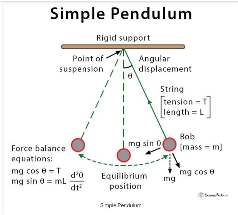
By applying Newton’s second law of motion for rotational systems, the equation of motion for the pendulum may be obtained

F=ma

`(d^2theta)/(dt^2)+b/m (d theta)/dt+g/lsintheta=0` eqn 1

Where,

g = gravity in m/s2,

L = length of the pendulum in m,

m = mass of the ball in kg,

b=damping coefficient.

substituting `theta=theta1`

`(d theta )/dt=(d theta1)/dt=theta2`

substitute in eqn 1

`(d theta )/dt=(d theta1)/dt=theta2`

we get,

`(d^2 theta1)/dt^2+b/m (d theta1)/dt+g/lsin theta1=0`

`(d theta2)/dt+b/m theta2+g/lsin theta1=0`

`(d theta2)/dt=- b/m theta2- g/lsin theta1`

solving ODE,

`(d theta1)/dt =theta2 |(d theta2)/dt =-b/m theta2-g/lsin theta1`

`(d)/dt [( theta1),(theta2)] =[(theta2),(-b/m theta2-g/l sin theta1)]`

CODE EXPLANATION :

STEP 1 : starting the matlab program with clear all removes all variables from the current workspace.close all colse all the figure window and clc clear the command window.

declaring the inputs given below

L=1 metre,

m=1 kg,

b=0.05.

g=9.81 m/s2.

STEP 2 : Initiating the intial condition defining angular displacement and velocity im rad/sec at time t=0.

Simulating the motion between 0-20 sec using the linspace command generates 200 values spacing between 0-20.

STEP 3 : Using the ODE45 function [t , result] =ode45(@(t,theta) ode_func(t,theta,b,g,l,m),time_span ,theta_0 ), where t_span = [0 20], integrates the system of differential equations y′=f(t,y) from 0 to 2 with initial conditions theta_0. Each row in the solution array y corresponds to a value returned in column vector t.

Specifying a time interval of theta_0 =[0 3] and the initial condition y0=0

ode_func is defined , Functions to solve, specified as a function handle that defines the functions to be integrated.

the ode_func is shown in below code

function [dtheta_dt] = ode_func(t,theta,b,g,l,m)
theta1 = theta(1)
theta2 =theta(2)
dtheta1_dt = theta2;
dtheta2_dt = -(b/m)*theta2-(g/l)*sin(theta1);
dtheta_dt = [dtheta1_dt ;dtheta2_dt];
end

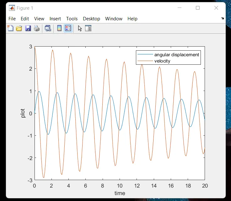
STEP 4 :plotting the graph to get the wave form of angular dispalcement and velocity in rad/sec figure 1

STEP 5:animating the transient motion of the simple pendulum using the for loop to repeat specified number of times

assuming ,

• One end of the pendulum is fixed i.e.(x0 y0) =(0 0)
• x1 =l*sin`theta` and y1 =-l*cos`theta`

plotting the graph for the animation of the simple pendulum

specifing the axis specifies the limits for the current axes.

pause Pause playback or recording to get good simulation of the pendulum.

getframe captures the current axes as it appears on the screen as a movie frame.

movie plays the movie frames in array M once. To create a movie frame from the current figure or axes, see getframe and compliles in .avi format

MATLAB CODE :

clear 
close all
clc
% program to solve ODE for a simple pendulum

%inputs
% damping coefficient
b = 0.05 ;
% gravity 9.81 m/s^2
g  =9.81;
% mass of the ball in kg
m = 1;
% length of the pendulum in m
l = 1;

% intial condition
% defining angular displacement and velocity im rad/sec at time t=0
theta_0 = [0;3];

% time points
time_span = linspace(0,20,200);

% To solve ODE
[t , result] =ode45(@(t,theta) ode_func(t,theta,b,g,l,m),time_span ,theta_0 );

%plotting
figure (1)

plot(t,result(:,1))
hold on
plot(t,result(:,2))
xlabel('time')
ylabel('plot')
legend('angular displacement','velocity')


% animating the transient motion of the simple pendulum
figure(2)
ct=1;

for i=1:length(result(:,1)) %for loop to repeat specified number of times
    
        x0 =0;
        y0 =0;

        x1 = l*sin(result(i,1));
        y1 =-l*cos(result(i,1));
      
       %plotting the graph
       plot([-1.5 1.5],[0 0])
       grid on
       hold on
       plot([x0 x1],[y0 y1],'linewidth',2,'Color','b') % creates the 2-D plot
       plot(x1,y1,'o','MarkerSize',22,'MarkerFaceColor',[1 1 0])
       axis([-1.5 1.5 -1.5 0.5])  % specifies the limits for the current axes
       pause(0.0003)     %Pause playback or recording
      
       M(ct) =getframe(gcf); %captures the current axes as it appears on the screen as a movie frame
       hold off
          ct=ct+1;
end
%  plays the movie frames in array M once. To create a movie frame from the current figure or axes, see getframe.
movie(M) 
Videofile = VideoWriter('second_ode.avi','Uncompressed AVI');
open(Videofile)
writeVideo(Videofile,M)
close(Videofile)

ERROR AND MEASURE FOR ERROR :

ERROR 1

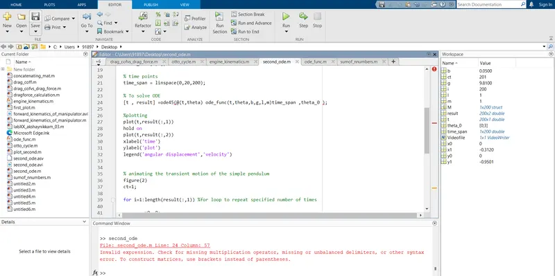
• The error was in line 24 while defining the t_span and the comma was missed after the ode_func
• this error was cleared by changing the t_span as intiated time_span and by providing the comma.

ERROR 2

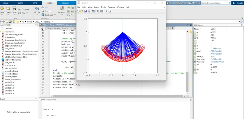
• The error was found as shown in above fig due to the hold on and hold off command and for the pause command .
• The error was cleared by using the proper value for the pause command and using the hold off command.

OUTPUT /RESULT :

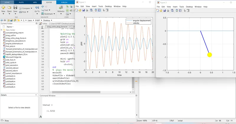
• The graph represent wave form of angular dispalcement and angular velocity w.r.t time
• From the graph we can conclude that displacement ,velocity,acceleration are periodic functions of time.

CONCLUSION :

Animation of the motion of pendulum is as shown , in the below link

https://www.youtube.com/watch?v=x-E3SwRQIs4