Week 4.1 - Genetic Algorithm
OBJECTIVES:
1. Write a code in MATLAB to optimise the stalagmite function and find the global maxima of the function.
2. Clearly explain the concept of genetic algorithm and also explain the syntax for ga in MATLAB.
3. Make sure that your code gives the same output, even if it is made to run several times.
4. Plot graphs for all 3 studies and for F maximum vs no. of iterations.
GENETIC ALGORITHM:
Genetic Algorithm(in MATLAB ga) is a solver used to search and calculate the global minima of a function. It is based on the Theory of Evolution proposed by Charles Darwin. As suggested, the solution of the problem comes after a number of generations or iterations. First generation/iteration of the possible solutions is tested for the objective function. The coming generations are derived from the previous generation solutions by selection, cross-over and mutation.
Selection is done by comparing against the fitness function values. In this process the solutions from both previous and current generation can be taken based on their fitness values. Cross-over is the merging or crossing of two solutions of current generation. Mutation is the modification of current generation solutions. Repeating these three processes over specified number of times/number of iterations allows the solution to converge and produce the output.
X = GA(FITNESSFCN,NVARS,A,b,Aeq,beq,lb,ub,NONLCON,INTCON,options)
This is the standard syntax for the ga solver. Here 'X' is the minimum of 'FITNESSFCN' function. Depending on the parameters, 'X' can be local or global minima. 'NVARS' is the number of design/input variables of the 'FITNESSFCN' function. 'A' and 'b' are the matrices formed from the inequalities of the linear constraints. 'Aeq' and 'Beq' are matrices generated from another set of linear inequalities. 'lb' and 'ub' are the lower and upper bounds on the design variables respectively. 'NONLCON' represents the non-linear inequalities. 'INTCON' forces the variables stored in it to take integer values. 'options' is used to modify/change the parameters values that are set by default.
GENETIC ALGORITHM CODE FOR GLOBAL OPTIMISATION:
%Global optimisaton by genetic algorithm method

%Range of x and y
x= linspace(0,0.6,150);
y= linspace(0,0.6,150);
%Number of iterations
num_cases=50;

%Mesh of x and y points
[xx,yy]= meshgrid(x,y);

%Calling of the stalagmite function
f=zeros(1,2);
s=zeros(1,2);
for i= 1:length(xx)
    for j= 1:length(yy)
        input_vector(1)= xx(i,j);
        input_vector(2)= yy(i,j);
        f(i,j)= stalagmite_mod(input_vector);
        s(i,j)= stalagmite(input_vector);
    end
end

%Generate surface plot
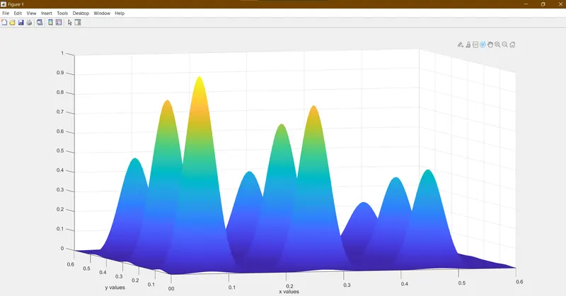
figure(1)
surf(xx,yy,s)
xlabel('x values')
ylabel('y values')
shading interp

%GA function
f_opt= zeros(1,50);
x_opt= zeros(1,50);
y_opt= zeros(1,50);
tic
for k=1:num_cases
    [inputs,f_opt(k)]= ga(@stalagmite_mod,2,[],[],[],[],[0,0],[0.25,0.25]);
        x_opt(k)= inputs(1);
        y_opt(k)= inputs(2);
end

%Plot
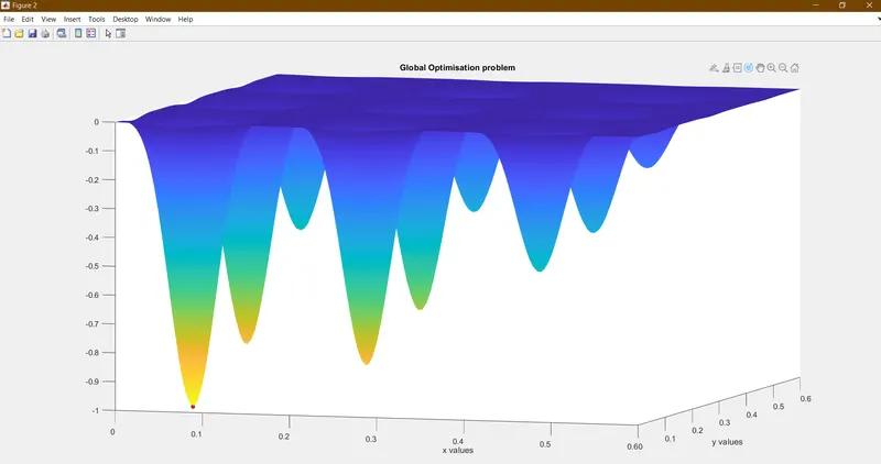
figure(2)
hold on
surf(xx,yy,f,-f)
xlabel('x values')
ylabel('y values')
shading interp
plot3(x_opt,y_opt,f_opt,'Marker','o','MarkerSize',5,'MarkerFaceColor','r')
title('Global Optimisation problem')
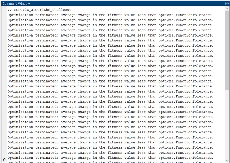
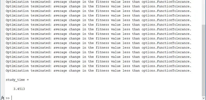
study_time= toc
EXPLANATION:
1. Comment
2.
3. Comment
4. Variable 'x' ranges from 0 to 0.6 with 150 values between 0 and 0.6.
5. Variable 'y' ranges from 0 to 0.6 with 150 values between 0 and 0.6.
6. Comment
7. The number of iterations/interactions of GA is assigned variable 'num_cases'=50.
8.
9. Comment
10. A 2D grid is created taking values of 'x' and 'y' with the help of 'meshgrid' command.
11.
12. Comment
13. Variable 'f' is pre allocated before for loop for better performance of the code.
14. Variable 's' is pre allocated before for loop for better performance of the code.
15. Start of for loop with count index variable 'i'.
16. Start of for loop with count index variable 'j'.
17. x-values of the meshgrid are assigned variable 'input_vector' in first element.
18. y-values of the meshgrid are assigned variable 'input_vector' in second element.
19. The x and y values of the meshgrid are taken as input for the modified stalagmite function from the 'input_vector' and result of the modified stalagmite function is assigned variable 'f'.
20. The x and y values of the meshgrid are taken as input for the stalagmite function from the 'input_vector' and result of the stalagmite function is assigned variable 's'.
21. End of second for loop.
22. End of first for loop.
23.
24. Comment
25. The command 'figure(1)' assigns the graphical commands to Figure1 window.
26. 'surf' command creates a surface in 3d using 'xx', 'yy' and 's' as x, y and z values respectively. This plots the standard stalagmite function in 3d.
27. 'xlabel' command assigns title to x-axis.
28. 'ylabel' command assigns title to y-axis.
29. 'shading interp' removes the wire mesh from the surface and shows the plot as colored and shaded.
30.
31. Comment
32. 'f_opt' is pre allocated before for loop for better performance of the code.
33. 'x_opt' is pre allocated before for loop for better performance of the code.
34. 'y_opt' is pre allocated before for loop for better performance of the code.
35. 'tic' is part of 'tic & toc' command which starts the timer for duration of running of the code.
36. Start of the for loop with count index variable 'k'.
37. The ga(genetic algorithm) command calculates the minima(optimal value) as 'f_opt' and its location as 'inputs' using the given function as fitness function. The area of inputs x and y is bounded from (0,0) to (0.25,0.25).
38. The first element of 'inputs' is assigned variable 'x_opt' which is the x-coordinate of the ga command output.
39. The second element of 'inputs' is assigned variable 'y_opt' which is the y-coordinate of the ga command output.
40. End of for loop.
41.
42. Command
43. 'figure(2)' assigns the graphical commands to Figure2 window.
44. 'hold on' command allows to show all plot commands on the same window.
45. 'surf' command creates a surface in 3d using 'xx', 'yy' and 'f' as x, y and z values respectively. The fourth matrix arguement is the scale of color shading in the plot.
46. 'xlabel' command assigns title to x-axis.
47. 'ylabel' command assigns title to y-axis.
48. 'shading interp' removes the wire mesh from the surface and shows the plot as colored and shaded.
49. 'plot3' command plots x,y,z values in 3d. 'Marker','MarkerSize','MarkerFaceColor' are scripts for customization so that plot is presentable.
50. 'title' command assigns a title to the plot.
51. 'tic & toc' command is ended with toc which completes the marker started with 'tic' command for the duration of running of the code.
OUTPUT:
STALAGMITE FUNCTION CODE:
%Stalagmite function code
function [f]= stalagmite(vector)

%f_1,x term
term1= (sin(15.70795.*vector(1)+0.5)).^6;
%f_1,y term
term2= (sin(15.70795.*vector(2)+0.5)).^6;
%f_2,x term
term3= exp(-4.33217.*((vector(1)-0.0667).^2));
%f_2,y term
term4= exp(-4.33217.*((vector(2)-0.0667).^2));

%f(x,y)= f_1,x.*f_1,y.*f_2,x.*f_2,y
f= term1.*term2.*term3.*term4;
end
EXPLANATION:
1. Comment
2. The function is assigned variable 'f' and named as 'stalagmite'. This function takes a variable/vector and gives the output as discussed further.
3.
4. Comment
5. The formula for f(1,x) term is assigned as variable 'term1'.
6. Comment
7. The formula for f(1,y) term is assigned as variable 'term2'.
8. Comment
9. The formula for f(2,x) term is assigned as variable 'term3'.
10. Comment
11. The formula for f(2,y) term is assigned as variable 'term4'.
12.
13. Comment
14. The formula for stalagmite function is divided into four terms and terms are calculated and substituted and assigned variable 'f' as the output of the function.
15. The end of the stalagmite function.
MODIFIED STALAGMITE FUNCTION CODE:
%Modified Stalagmite function code
function [f]= stalagmite_mod(vector)

%f_1,x term
term1= (sin(15.70795.*vector(1)+0.5)).^6;
%f_1,y term
term2= (sin(15.70795.*vector(2)+0.5)).^6;
%f_2,x term
term3= exp(-4.33217.*((vector(1)-0.0667).^2));
%f_2,y term
term4= exp(-4.33217.*((vector(2)-0.0667).^2));

%f(x,y)= -f_1,x.*f_1,y.*f_2,x.*f_2,y
f= -term1.*term2.*term3.*term4;
end
EXPLANATION:
1. Comment
2. The function is assigned variable 'f' and named as 'stalagmite_mod'. This function takes a variable/vector and gives the output as discussed further. This is a modification of the standard 'stalagmite' function.
3.
4. Comment
5. The formula for f(1,x) term is assigned as variable 'term1'.
6. Comment
7. The formula for f(1,y) term is assigned as variable 'term2'.
8. Comment
9. The formula for f(2,x) term is assigned as variable 'term3'.
10. Comment
11. The formula for f(2,y) term is assigned as variable 'term4'.
12.
13. Comment
14. The formula for modified stalagmite function is divided into four terms and terms are calculated and substituted and assigned variable 'f' as the output of the function. A negative sign is added as modification for the stalagmite function.
15. The end of the modified stalagmite function.
GENETIC ALGORITHM STUDY CODE:
%Study of genetic algorithm optimisation problem

%Range of x and y
x= linspace(0,0.6,150);
y= linspace(0,0.6,150);
%Number of iterations
num_cases=50;

%Mesh of x and y points
[xx,yy]= meshgrid(x,y);

%Calling of the stalagmite function
f=zeros(1,2);
for i= 1:length(xx)
    for j= 1:length(yy)
        input_vector(1)= xx(i,j);
        input_vector(2)= yy(i,j);
        f(i,j)= stalagmite_mod(input_vector);
    end
end


%Study 1: Statistical behaviour
f_opt1= zeros(1,50);
x_opt1= zeros(1,50);
y_opt1= zeros(1,50);
tic
for k= 1:num_cases
    [inputs1,f_opt1(k)]= ga(@stalagmite_mod,2);
    x_opt1(k)= inputs1(1);
    y_opt1(k)= inputs1(2);
end

%Study 1 plot
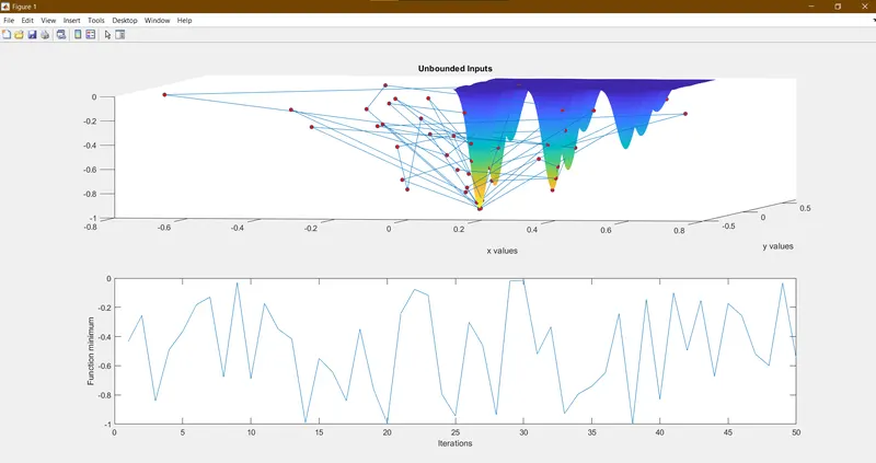
figure(1)
subplot(2,1,1)
hold on
surf(x,y,f,-f)
xlabel('x values')
ylabel('y values')
shading interp
plot3(x_opt1,y_opt1,f_opt1,'Marker','o','MarkerSize',5,'MarkerFaceColor','r')
title('Unbounded Inputs')
subplot(2,1,2)
plot(f_opt1)
xlabel('Iterations')
ylabel('Function minimum')
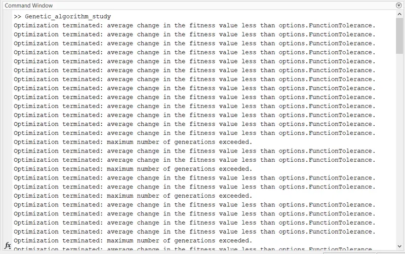
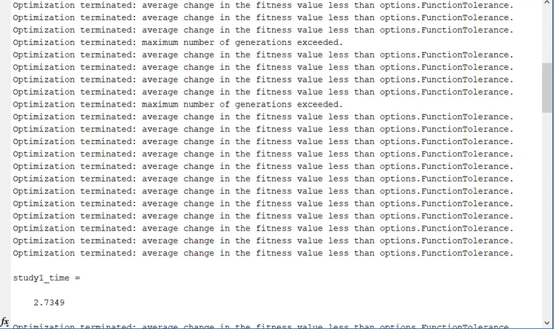
study1_time=toc

%Study 2: Statistical behaviour with upper and lower bounds
f_opt2= zeros(1,50);
x_opt2= zeros(1,50);
y_opt2= zeros(1,50);
tic
for l=1:num_cases
    [inputs2,f_opt2(l)]= ga(@stalagmite_mod,2,[],[],[],[],[0,0],[1,1]);
    x_opt2(l)= inputs2(1);
    y_opt2(l)= inputs2(2);
end

%Study 2 plot
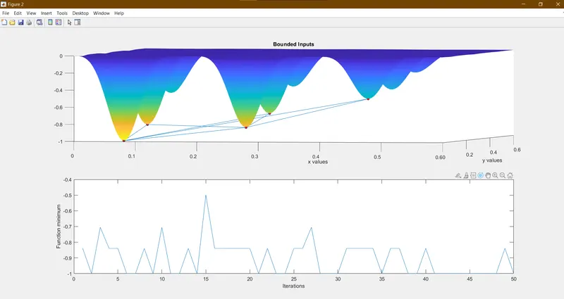
figure(2)
subplot(2,1,1)
hold on
surf(x,y,f,-f)
xlabel('x values')
ylabel('y values')
shading interp
plot3(x_opt2,y_opt2,f_opt2,'Marker','o','MarkerSize',5,'MarkerFaceColor','r')
title('Bounded Inputs')
subplot(2,1,2)
plot(f_opt2)
xlabel('Iterations')
ylabel('Function minimum')
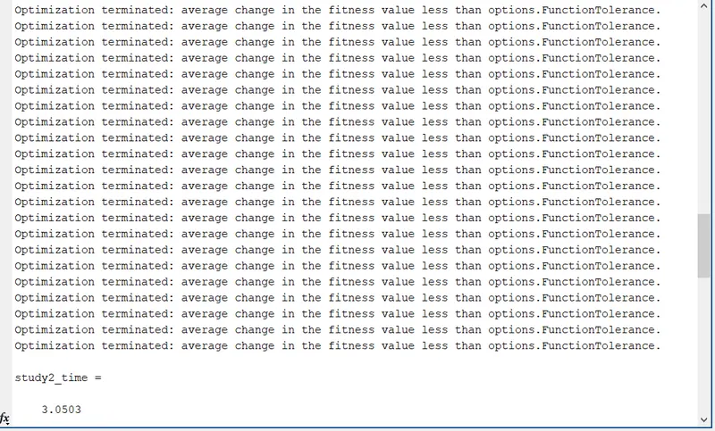
study2_time=toc

%Study 3: Increasing GA interactions
options= optimoptions('ga');
options= optimoptions(options,'PopulationSize',170);
f_opt3= zeros(1,50);
x_opt3= zeros(1,50);
y_opt3= zeros(1,50);
tic
for m= 1:num_cases
    [inputs3,f_opt3(m)]= ga(@stalagmite_mod,2,[],[],[],[],[0,0],[1,1],[],[],options);
    x_opt3(m)= inputs3(1);
    y_opt3(m)= inputs3(2);
end

%Study 3 plot
figure(3)
subplot(2,1,1)
hold on
surf(x,y,f,-f)
xlabel('x values')
ylabel('y values')
shading interp
plot3(x_opt3,y_opt3,f_opt3,'Marker','o','MarkerSize',5,'MarkerFaceColor','r')
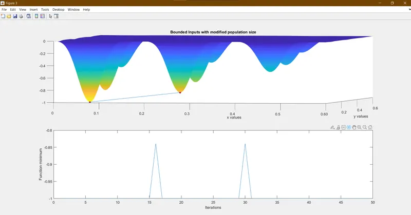
title('Bounded Inputs with modified population size')
subplot(2,1,2)
plot(f_opt3)
xlabel('Iterations')
ylabel('Function minimum')
study3_time=toc
EXPLANATION:
1. Comment
2.
3. Comment
4. Variable 'x' ranges from 0 to 0.6 with 150 values between 0 and 0.6.
5. Variable 'y' ranges from 0 to 0.6 with 150 values between 0 and 0.6.
6. Comment
7. The number of iterations/interactions of GA is assigned variable 'num_cases'=50.
8.
9. Comment
10. A 2D grid is created taking values of 'x' and 'y' with the help of 'meshgrid' command.
11.
12. Comment
13. Variable 'f' is pre allocated before for loop for better performance of the code.
14. Start of for loop with count index variable 'i'.
15. Start of for loop with count index variable 'j'.
16. x-values of the meshgrid are assigned variable 'input_vector' in first element.
17. y-values of the meshgrid are assigned variable 'input_vector' in second element.
18. The x and y values of the meshgrid are taken as input for the modified stalagmite function from the 'input_vector' and result of the modified stalagmite function is assigned variable 'f'.
19. End of second for loop.
20. End of first for loop.
21.
22.
23. Comment
24. Variable 'f_opt1' is pre allocated for better performance of the code.
25. Variable 'x_opt1' is pre allocated for better performance of the code.
26. Variable 'y_opt1' is pre allocated for better performance of the code.
27. 'tic' is part of 'tic & toc' command which starts the timer for duration of running of the code.
28. Start of for loop with count index variable 'k'.
29. 'ga' command calculates the minima of the given function and shows the output as 'inputs1' and 'f_opt1'.
30. The first element of 'inputs1' is assigned variable 'x_opt1'.
31. The second element of 'inputs1' is assigned variable 'y_opt1'.
32. End of for loop.
33.
34. Comment
35. The command 'figure(1)' assigns the graphical commands to Figure1 window.
36. 'subplot' command allows multiple graphs/plots to show in the same figure window. It divides the figure window into a matrix of first two arguements and select one of the elements and assigns later graphical commands to it.
37. 'hold on' command allows to show all plot commands on the same window.
38. 'surf' command creates a surface in 3d using 'xx', 'yy' and 'f' as x, y and z values respectively. The fourth matrix arguement is the scale of color shading in the plot.
39. 'xlabel' command assigns title to x-axis.
40. 'ylabel' command assigns title to y-axis.
41. 'shading interp' removes the wire mesh from the surface and shows the plot as colored and shaded.
42. 'plot3' command plots x,y,z values in 3d. 'Marker','MarkerSize','MarkerFaceColor' are scripts for customization so that plot is presentable.
43. 'title' command assigns a title to the plot.
44. The second element in the plot matrix is accessed by 'subplot' command.
45. Output of the ga is plotted.
46. 'xlabel' command assigns title to x-axis.
47. 'ylabel' command assigns title to y-axis.
48. 'tic & toc' command is ended with toc which completes the marker started with 'tic' command for the duration of running of the code.
49.
50. Comment
51. Variable 'f_opt2' is pre allocated for better performance of the code.
52. Variable 'x_opt2' is pre allocated for better performance of the code.
53. Variable 'y_opt2' is pre allocated for better performance of the code.
54. 'tic' is part of 'tic & toc' command which starts the timer for duration of running of the code.
55. Start of for loop with count index variable 'l'.
56. 'ga' command calculates the minima of the given function and shows the output as 'inputs2' and 'f_opt2'. The inputs are bounded from (0,0) to (1,1).
57. The first element of 'inputs2' is assigned variable 'x_opt2'.
58. The second element of 'inputs2' is assigned variable 'y_opt2'.
59. End of for loop.
60.
61. Comment
62. The command 'figure(2)' assigns the graphical commands to Figure2 window.
63. 'subplot' command allows multiple graphs/plots to show in the same figure window. It divides the figure window into a matrix of first two arguements and select one of the elements and assigns later graphical commands to it.
64. 'hold on' command allows to show all plot commands on the same window.
65. 'surf' command creates a surface in 3d using 'xx', 'yy' and 'f' as x, y and z values respectively. The fourth matrix arguement is the scale of color shading in the plot.
66. 'xlabel' command assigns title to x-axis.
67. 'ylabel' command assigns title to y-axis.
68. 'shading interp' removes the wire mesh from the surface and shows the plot as colored and shaded.
69. 'plot3' command plots x,y,z values in 3d. 'Marker','MarkerSize','MarkerFaceColor' are scripts for customization so that plot is presentable.
70. 'title' command assigns a title to the plot.
71. The second element in the plot matrix is accessed by 'subplot' command.
72. Output of the ga is plotted.
73. 'xlabel' command assigns title to x-axis.
74. 'ylabel' command assigns title to y-axis.
75. 'tic & toc' command is ended with toc which completes the marker started with 'tic' command for the duration of running of the code.
76.
77. Comment
78. 'optimoptions' is used to modify the options/parameter conditions for the solver as mentioned in the brackets.
79. 'options' for the command/solver 'ga' is changed with new parameter(populationSize=170).
80. Variable 'f_opt3' is pre allocated for better performance of the code.
81. Variable 'x_opt3' is pre allocated for better performance of the code.
82. Variable 'y_opt3' is pre allocated for better performance of the code.
83. 'tic' is part of 'tic & toc' command which starts the timer for duration of running of the code.
84. Start of the for loop with count index variable 'm'.
85. 'ga' command calculates the minima of the given function and shows the output as 'inputs2' and 'f_opt2'. The inputs are bounded from (0,0) to (1,1). The default paramter values are changed by 'options'.
86. The first element of 'inputs3' is assigned variable 'x_opt3'.
87. The second element of 'inputs3' is assigned variable 'y_opt3'.
88. End of for loop.
89.
90. Comment
91. The command 'figure(3)' assigns the graphical commands to Figure2 window.
92. 'subplot' command allows multiple graphs/plots to show in the same figure window. It divides the figure window into a matrix of first two arguements and select one of the elements and assigns later graphical commands to it.
93. 'hold on' command allows to show all plot commands on the same window.
94. 'surf' command creates a surface in 3d using 'xx', 'yy' and 'f' as x, y and z values respectively. The fourth matrix arguement is the scale of color shading in the plot.
95. 'xlabel' command assigns title to x-axis.
96. 'ylabel' command assigns title to y-axis.
97. 'shading interp' removes the wire mesh from the surface and shows the plot as colored and shaded.
98. 'plot3' command plots x,y,z values in 3d. 'Marker','MarkerSize','MarkerFaceColor' are scripts for customization so that plot is presentable.
99. 'title' command assigns a title to the plot.
100. The second element in the plot matrix is accessed by 'subplot' command.
101. Output of the ga is plotted.
102. 'xlabel' command assigns title to x-axis.
103. 'ylabel' command assigns title to y-axis.
104. 'tic & toc' command is ended with toc which completes the marker started with 'tic' command for the duration of running of the code.
OUTPUT:
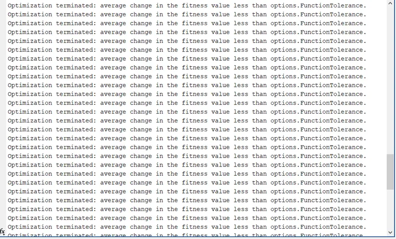
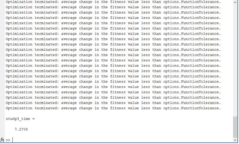
REFERENCES:
1. https://skill-lync.com/knowledgebase/genetic-algorithm-explained