Week 3 - Solving second order ODEs
AIM:
Solve for the motion of simple pendulum in MATLAB.
EQUATION:
d^2(theta)/dt^2 + (b/m)*(d(theta)/dt)+(g/L)*sin(theta)=0
where, g = acceleration due to gravity(m/s^2)
L = length of the pendulum(m)
m = mass of the ball(kg)
b= damping coefficient
theta= angular displacement from mean position
OBJECTIVE:
1. Solve the second-order differential equation.
2. Simulate the pendulum motion.
MAIN CODE:
%Motion of a simple pendulum described with the help of ODE

%Given quantites
%Acceleration due to gravity(m/sec^2)
g= 9.81;
%Length of pendulum(m)
l= 1;
%Mass of pendulum ball(kg)
m=1;
%Damping coefficient
b=0.05;

%Intial conditions
%Angular displacement= 0 radian
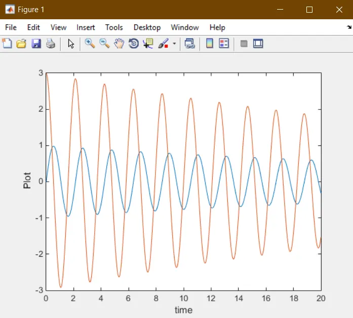
%Angular velocity= 3 radian/sec
theta_0= [0;3];

%Time
t_span= linspace(0,20,500);

%Solution ODE
[t,results]= ode45(@(t,theta) ode_func(t,theta,b,g,l,m),t_span,theta_0);

%For graph of displacement and velocity
figure(1)
plot(t,results(:,1))
hold on
plot(t,results(:,2))
xlabel('time')
ylabel('Plot')

%For simple pendulum animation figure window
x0=0;
y0=0;
ct=1;
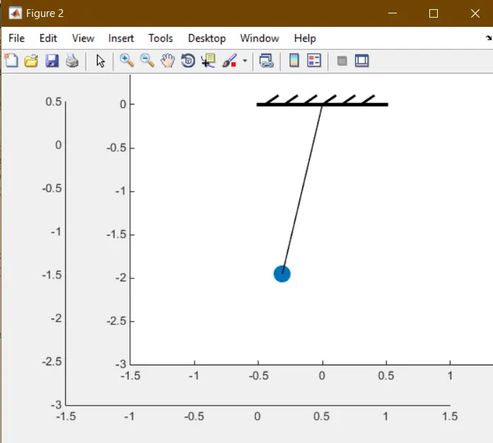
for i=1:length(t_span);
    %for loop for different positions of pendulum
    theta_sol= results(i,1);
    x_coordinate= sin(theta_sol);
    y_coordinate= 1-cos(theta_sol)-2;
    figure(2)
    %Marker representing mass/ball of pendulum
    plot(x_coordinate,y_coordinate,'Marker','.','MarkerSize',50)
    %Line representing string/chord of pendulum
    line([x0 x_coordinate],[y0 y_coordinate],'linewidth',1,'color','k')
    %Lines representing fixed wall
    line([-0.5 0.5],[0 0],'linewidth',3,'color','k')
    line([-0.45 0.-0.35],[0 0.1],'linewidth',2,'color','k')
    line([-0.3 0.-0.2],[0 0.1],'linewidth',2,'color','k')
    line([-0.15 0.-0.05],[0 0.1],'linewidth',2,'color','k')
    line([0 0.1],[0 0.1],'linewidth',2,'color','k')
    line([0.15 0.25],[0 0.1],'linewidth',2,'color','k')
    line([0.3 0.4],[0 0.1],'linewidth',2,'color','k')
    axis([-1.5 1.5 -3 0.5])
    pause(0.02)
    %For storing images/frames for video
    M(ct)=getframe(gcf);
    ct=ct+1;
end
%end of for loop

%Video file of plot
movie(M)
videofile=VideoWriter('Simple_pendulum_ODE_challenge.avi','Uncompressed AVI');
open(videofile)
writeVideo(videofile,M)
close(videofile)
EXPLANATION:
1. Comment
2.
3. Comment
4. Comment
5. Variable 'g' is the acceleration due to gravity(9.81 m/sec^2)
6. Comment
7. Length of pendulum is assigned variable 'l'(1 m).
8. Comment
9. Variable 'm' is assigned to mass of the pendulum(1 kg).
10. Comment
11. Damping coefficient(0.05) is stored as variable 'b'.
12.
13. Comment
14. Comment
15. Comment
16. Intial condition matrix is a column matrix assigned as 'theta_0'.
17.
18. Comment
19. Time is taken from 0 to 20 seconds. A large number of values are necessary for simple pendulum. The variable is t_span.
20.
21. Comment
22. The syntax for simple pendulum can be compared to the standard syntax of ode45 and explained. [t,y]=ode45(@(t,y),func(t,y),t_span,conditions).HEre, the variable y is the matrix 'theta'. Conditions refers to the conditions required to solve the ODE.
23.
24. Comment
25. figure(1) designates the next commands of plot to Figure1 window.
26. This plot command plots time vs angular displacement of the pendulum which is the solution of the ODE. 'results(:,1)' takes all the values from all rows and 1st column of the matrix.
27. hold on command retrieves all the plots in the figure.
28. This plot command plots velocity against time in the figure.
29. 'xlabel' designates the title of x-axis.
30. 'ylabel' designates the title of y-axis.
31.
32. Comment
33. Abscissa of reference point is taken as x0=0.
34. Ordinate of reference point is taken as y0=0.
35. Variable 'ct' is pre-allocated.
36. for loop is initiated with index 'i'. 'i' ranges from 1 to length of 't_span' i.e. 500.
37. Comment
38. The solution of ODE(i.e. angular displacement) is given a new variable 'theta_sol'.
39. For the plot which gives position of the mass of pendulum, its coordinates are needed. By simple geometry, x-coordinate can be given by sin(angular displacement).
40. y-coordinate is given by 1-cos(angular displacement). 2 is subtracted from y coordinate for the sake of presentability.
41. figure(2) designates the next set of commands to the Figure2 window.
42. Comment
43. This plot represents the position of the mass of pendulum. It is defined by x and y coordinates. Marker defines the shape of the point which is a solid circle and MarkerSize defines the size of the Marker.
44. Comment
45. Since 'plot' and 'hold on' commands cannot be used here thus line command is used to plot the remaining simple pendulum. This line command represnts the cord of the pendulum to which mass is attached.
46. Comment
47. The chord is attached to a fixed support. Hence this line command represents the boundary of the fixed support/wall.
48. This line command completes the pictorial representation of the fixed wall.
49. This line command completes the pictorial representation of the fixed wall.
50. This line command completes the pictorial representation of the fixed wall.
51. This line command completes the pictorial representation of the fixed wall.
52. This line command completes the pictorial representation of the fixed wall.
53. This line command completes the pictorial representation of the fixed wall.
54. The range of the axes is designated with the help of 'axis' command. First start and end x-coordinates are defined and then start and end y-coordinate are defined.
55. pause(n) command pauses the running of the code for n seconds and waits user response. In this case, no such response is needed.
56. Comment
57. The 'getframe' command takes a snapshot of the current plot and returns it into a movie frame. With for loop, 'getframe' can be used to assemble many such frames for playback.
'gcf' returns the handle of current figure. With 'getframe' command, the stored handle of the figure can be queried directly. In this case, 'M' variable stores the figures obtained by 'gcf' and 'getframe'.
58. For all the figures/frames to be stored in the variable 'M', it is necessary for 'ct' to progress with every instance of for loop, thus every time a plot is done, it is converted to frame and stored in 'M', thus 'ct' needs to be incremented.
59. for loop is ended here.
60. Comment
61.
62. Comment
63. 'movie(s)' command plays the frames/array of frames stored in the variable s. This command works together with 'getframe' and 'gcf' to create a video. The variable s needs to be an array of movie frames.
64. 'VideoWriter' command constructs a VideoWriter object to write video data to an AVI file that uses Motion JPEG compression. The set of properties such as compressed or uncompressed can be changed by specifying a profile set.
65. 'open' command opens the file for changes, editing or writing.
66. 'writeVideo' writes the file(in this case video file) after the 'open' command with the help of Video Writer. In this case it uses the variable 'M' which already has frames stored in it.
67. 'close(videofile)' completes the code after open and write operations. It is necessary to close the file to save the frames otherwise the video file will not be saved and will show void.
FUNCTION CODE:
%Function to solve ODE of simple pendulum
function [dtheta_dt]= ode_func(t,theta,b,g,l,m)

%Variable matrix theta
theta1= theta(1);
theta2= theta(2);
dtheta1_dt= theta2;
%Equations obtained by replacing dtheta1/dt by theta2
dtheta2_dt= -(b/m)*theta2-(g/l)*sin(theta1);
dtheta_dt= [dtheta1_dt; dtheta2_dt];

end
EXPLANATION:
1. Comment
2. To solve an ODE, a function is necessary to call and assign variables to equations for ode45 to solve.
3.
4. Comment
5. The first element of theta, i.e. theta(1) is assigned a variable 'theta1'.
6. The second element of theta, i.e. theta(2) is assigned variable 'theta2'.
7. To solve ODE, differentiation of theta with respect to time is designated as theta2. Replacing 'dtheta1/dt' by 'theta2' in the equations turns a second order differential equation into first order differential.
8. Comment
9. The second order equation converted into first order.
10. Comment
11. The solution matrix theta is obtained by defining its elements.
12.
13. Termination of the function.
OUTPUT:
https://drive.google.com/file/d/1zIGJHkU_O6NONc16EMrHNTeSg-HK4qJZ/view?usp=sharing
ERRORS:
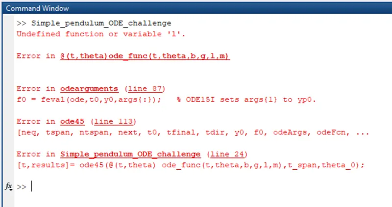
1. Using an undefined variable in ode45.
2. Not using comma in the syntax of plot command.
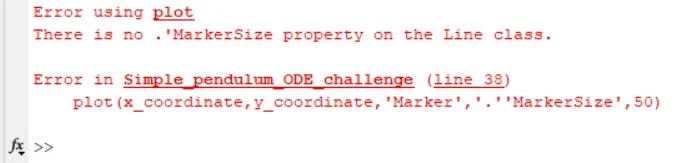
SOLUTION:
1. Change variable from 'L' to 'l'.
2. Putting comma in between '.' and 'MarkerSize'.