Week 4.1 - Genetic Algorithm

Aim:

To Write a code in MATLAB to optimise the stalagmite function and find the global maxima of the function.

Given:

f1,x=[sin(5.1pix + 0.5)]^6

f1,y=[sin(5.1piy + 0.5)]^6

f2,x=exp[-4log(2)(x-0.0667)^2/0.64]

f2,y=exp[-4log(2)(y-0.0667)^2/0.064]

`f(x,y)=f1,x.f2,x.f1,y.f2,y`

objectives:

The main operators of the genetic algorithms are reproduction, crossover, and mutation. Reproduction is a process based on the objective function (fitness function) of each string. This objective function identifies how “good” a string is.They are commonly used to generate high-quality solutions for optimization problems and search problems. Genetic algorithms simulate the process of natural selection which means those species who can adapt to changes in their environment are able to survive and reproduce and go to next generation.

Introduction:

OPTIMIZATION:

When you optimize something, you are “making it best”. “Optimization” comes from the same root as “optimal”, which means best. When you optimize something, you are “making it best”. The objective function, f(x), which is the output you're trying to maximize or minimize.

example-If you’re a football player,you might want to maximize your running yards, and also minimize your fumbles. Both
maximizing and minimizing are types of optimization problems.

OPTIMIZATION PROCESS:

• His main goal is to maximize running yards – this will become his objective function.
• He can make his athletes spend practice time in the weightroom; running sprints; or practicing ball protection. The amount of time spent on each is a variable (by varying the parameters).
• However, there are limits to the total amount of time he has. Also, if he completely sacrifices ball protection he may
  see running yards go up, but also fumbles, so he may place an upper limit on the amount of fumbles he considers acceptable. These are constraints.

Genetic Algorithm:

A genetic algorithm is a search based algorithm that is inspired by Charles Darwin’s theory of natural evolution. This algorithm reflects the process of natural selection where the fittest individuals are selected for reproduction in order to produce offspring of the next generation.

Natural selection:

The process of natural selection starts with the selection of fittest individuals from a population. They produce offspring which inherit the characteristics of the parents and will be added to the next generation. If parents have better fitness, their offspring will be better than parents and have a better chance at surviving. This process keeps on iterating and at the end, a generation with the fittest individuals will be found.

Five phases are considered in a genetic algorithm.

• Initial population
• Fitness function
• Selection
• Crossover
• Mutation

Inital population.

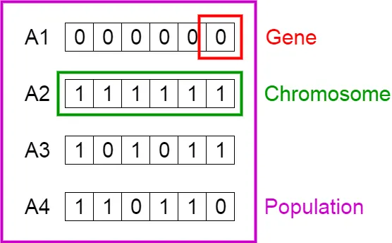
The process begins with a set of individuals which is called a Population. Each individual is a solution to the problem you want to solve. An individual is characterized by a set of parameters (variables) known as Genes. Genes are joined into a string to form a Chromosome (solution). In a genetic algorithm, the set of genes of an individual is represented using a string, in terms of an alphabet. Usually, binary values are used (string of 1s and 0s). We say that we encode the genes in a chromosome.

Fitness function:

The fitness function determines how fit an individual is (the ability of an individual to compete with other individuals). It gives a fitness score to each individual. The probability that an individual will be selected for reproduction is based on its fitness score.

Selection:

The idea of selection phase is to select the fittest individuals and let them pass their genes to the next generation.Two pairs of individuals (parents) are selected based on their fitness scores. Individuals with high fitness have more chance to be selected for reproduction.

Cross over:

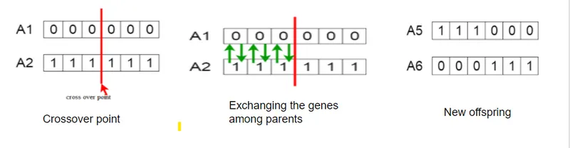
Crossover is the most significant phase in a genetic algorithm. For each pair of parents to be mated, a crossover point is chosen at random from within the genes.For example, consider the crossover point to be 3 as shown below.

Mutation:

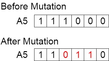
In certain new offspring formed, some of their genes can be subjected to a mutation with a low random probability. This implies that some of the bits in the bit string can be flipped.Mutation occurs to maintain diversity within the population and prevent premature convergence.

Termination:

The algorithm terminates if the population has converged (does not produce offspring which are significantly different from the previous generation). Then it is said that the genetic algorithm has provided a set of solutions to our problem.

GA syntax in matlab:

• x = ga(fun,nvars)

fun=function handle or function name

• nvars=no. of variables

x = ga(fun,nvars,A,b)

• A=linear inequality consraints,specifid as real matrix.
• b=linear inequality consraints,specifid as real vector.

x = ga(fun,nvars,A,b,Aeq,beq)

• Aeq=linear equalities of A
• beq=linear equalities of b

x = ga(fun,nvars,A,b,Aeq,beq,lb,ub)

• lb=lower bound
• ub=upper bound

x = ga(fun,nvars,A,b,Aeq,beq,lb,ub,nonlcon)

• nonlcon=non linear constrains specified as function handle or function name

x = ga(fun,nvars,A,b,Aeq,beq,lb,ub,nonlcon,options)

• options=optimization options,specified as output optimization.

x = ga(fun,nvars,A,b,Aeq,beq,lb,ub,nonlcon,intcon)

• intcoin=ingeger variable.

x = ga(fun,nvars,A,b,Aeq,beq,lb,ub,nonlcon,intcon,options)

x=ga(problem)

• ga(problem)=problem description described as structure.

[x,fval]=ga(___)

• return the value of fitness function x

[x,fval,exitflag,output]=ga(___)

• exitflag=Where there are integier constrains,ga use the penality fitness value instead of fitness value for stopping criteria.

[x,fval,exitflag,output,population,scores]=ga(___)

• population=final population returned as population size.
• scores=scores are penality fitness value of the population members.

program.1

• Write a code in MATLAB to optimise the stalagmite function and find the global maxima of the function.
• Make sure that your code gives the same output, even if it is made to run several times.
• Plot graphs for all 3 studies and for F maximum vs no. of iterations. Title and axes labels are a must, legends could be shown if necessary.

clear all
close all
clc

% Inputs used for search space
x =linspace(0,0.6,150);
y =linspace(0,0.6,150);

% creating the 2d dimensionl mesh
[xx yy]=meshgrid(x,y);

% evaluating the staglimite function & calling the function stalagmite
tic
num_cases =50;
for i =1:length(xx);
    for j=1:length(yy)
        input_vector(1)=xx(i,j);
        input_vector(2)=yy(i,j);
        f(i,j) =stalagmite(input_vector);
    end
end
% study1 statical behaviors 
tic
for i=1:num_cases
    [inputs, fopt(i)] =ga(@stalagmite,2);
  xopt(i)= inputs(1);
  yopt(i)=inputs(2);
end
calculation1_time =toc
figure(1)
subplot(2,1,1);
surf(x,y,-f);
shading interp
hold on
plot3(xopt,yopt,-fopt,'marker','o','MarkerSize',4,'MarkerFaceColor','r');
title('unboundedinputs')
subplot(2,1,2);
plot(-fopt);
xlabel('function iteration');
ylabel('function maxima');


% statical behavior with upper and lower bound
tic
for i= 1:num_cases;
    [inputs,fopt(i)] =ga(@stalagmite,2,[],[],[],[],[0;0],[1;0.6]);
    xopt(i)=inputs(1);
    yopt(i)=inputs(2);
end

calculation2_time= toc
figure(2)
subplot(2,1,1);
surf(x,y,-f);
hold on
shading interp
plot3(xopt,yopt,-fopt,'marker','o','MarkerSize',4,'MarkerFaceColor','r');
title('unboundedinputs')
subplot(2,1,2);
plot(-fopt);
xlabel('function iteration');
ylabel('function minimum');


% Increase the initial population
tic
options=optimoptions("ga")
options =optimoptions(options,'PopulationSize',250);
for i= 1:num_cases;
    [inputs,fopt(i)] =ga(@stalagmite,2,[],[],[],[],[0,0],[0.6,0.6],[],[],options);
    xopt(i)=inputs(1);
    yopt(i)=inputs(2);
end
calculation3_time= toc
figure(3)
subplot(2,1,1);
surf(x,y,-f);
hold on
shading interp
plot3(xopt,yopt,-fopt,'marker','o','MarkerSize',4,'MarkerFaceColor','r');
title('boundedinputs')
subplot(2,1,2);
plot(-fopt);
xlabel('function iteration');
ylabel('function minimum');
tic

• I take no of iteration is 50 and we store our outputs into results which contains maximas and fopt contains at which values The maxima is obtained.ga(@stalagmite,2) in calling function we use 2 because in function we having 2 variables so we provide it to the ga.
• Tic and toc is used to calculate the program run time it would be show in command window.
• When my results has been stored in xopt & yopt. and fopt shows the values of maxima is obtained.
• Now we stores the results and values of xopt,yopt and fopt, we need to plot that on the surface (x,y,-f)
• using the surfc command (x,y,-f) we got the 3D view of plots. we can plot the results and values of (xopt,yopt,-fopt) on that surface so we can use he hold on command to explore the both plots
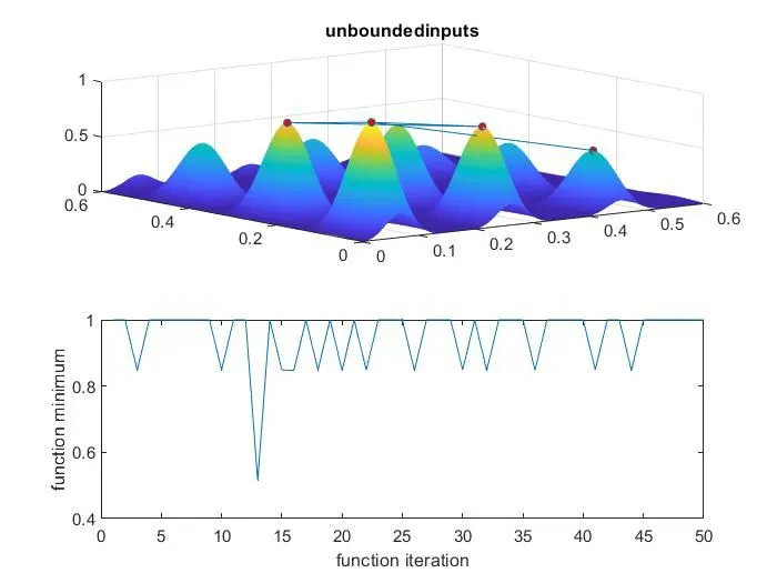
• using the subplot command we can take a set a order of two different plot of image in 1 figure to !st sub plot mentioned as to visualize maxima plot the results and values on that the 2nd sub plot mentioned as check the boundries with respect to iteration.the output has been mentioned below

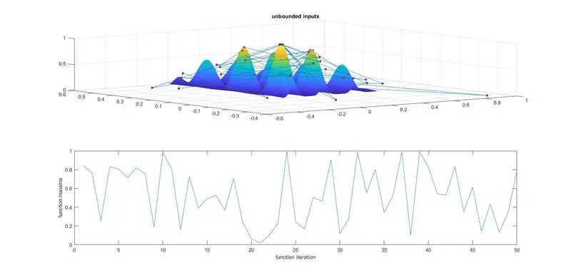
so,In this figure the optimal values went outside the value of x and y resulting in falling away from the satalagmite surface. so in this case to reach the global maxima is failed.

now let us maker our study with bounded values.

Let us specify the lower and upper bounds of x and y,still the ga initated with random population only.

tic
for i= 1:num_cases;
[inputs,fopt(i)] =ga(@stalagmite,2,[],[],[],[],[0;0],[1;0.6]);
xopt(i)=inputs(1);
yopt(i)=inputs(2);
end

calculation2_time= toc
figure(2)
subplot(2,1,1);
surf(x,y,-f);
hold on
shading interp
plot3(xopt,yopt,-fopt,'marker','o','MarkerSize',4,'MarkerFaceColor','r');
title('unboundedinputs')
subplot(2,1,2);
plot(-fopt);
xlabel('function iteration');
ylabel('function minimum');

• I take no of iteration is 50 and we store our outputs into results which contains maximas and fopt contains at which values The maxima is obtained.ga(@stalagmite,2) in calling function we use 2 because in function we having 2 variables so we provide it to the ga.
• Tic and toc is used to calculate the program run time it would be show in command window.
• When my results has been stored in xopt & yopt. and fopt shows the values of maxima is obtained.
• Now we stores the results and values of xopt,yopt and fopt, we need to plot that on the surface (x,y,-f)
• using the surfc command (x,y,-f) we got the 3D view of plots. we can plot the results and values of (xopt,yopt,-fopt) on that surface so we can use he hold on command to explore the both plots
• using the subplot command we can take a set a order of two different plot of image in 1 figure to 1st sub plot mentioned as to visualize maxima plot the results and values on that the 2nd sub plot mentioned as check the boundries with respect to iteration.the output has been mentioned below

in this figure the optimim value are within the boundries limits but still it could not show exact maxima value.

Now let us make our study with initial population and bounded values

In this case let us increase our initial population which is default at 50 to 250

% Increase the initial population
tic
options=optimoptions("ga")
options =optimoptions(options,'PopulationSize',250);
for i= 1:num_cases;
[inputs,fopt(i)] =ga(@stalagmite,2,[],[],[],[],[0,0],[0.6,0.6],[],[],options);
xopt(i)=inputs(1);
yopt(i)=inputs(2);
end
calculation3_time= toc
figure(3)
subplot(2,1,1);
surf(x,y,-f);
hold on
shading interp
plot3(xopt,yopt,-fopt,'marker','o','MarkerSize',4,'MarkerFaceColor','r');
title('boundedinputs')
subplot(2,1,2);
plot(-fopt);
xlabel('function iteration');
ylabel('function minimum');
tic

Here in this case to set a initial population we need to use command called optimum option get over the population size to 250.

• I take no of iteration is 50 and we store our outputs into results which contains maximas and fopt contains at which values The maxima is obtained.ga(@stalagmite,2) in calling function we use 2 because in function we having 2 variables so we provide it to the ga.
• Tic and toc is used to calculate the program run time it would be show in command window.
• When my results has been stored in xopt & yopt. and fopt shows the values of maxima is obtained.
• Now we stores the results and values of xopt,yopt and fopt, we need to plot that on the surface (x,y,-f)
• using the surfc command (x,y,-f) we got the 3D view of plots. we can plot the results and values of (xopt,yopt,-fopt) on that surface so we can use he hold on command to explore the both plots
• using the subplot command we can take a set a order of two different plot of image in 1 figure to 1st sub plot mentioned as to visualize maxima plot the results and values on that the 2nd sub plot mentioned as check the boundries with respect to iteration.the output has been mentioned below.

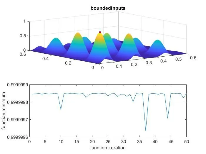
Here we finally got the results,in this figure we got the correct maxima values for the stalagmite function.by increasing the initial population size of the ga we can get the accuracy of algorithm