Curve fitting by unsing linear and cubic polynomial

Aim:

Write a code to show the different types of curvce fitting polynomial.

Objectives:

1. Write code to fit a linear and cubic polynomial for the Cp data.
2. Plot the linear and cubic fit curves along with the raw data points. Title and axes labels are a must, legends could be shown if necessary.
3. Write a code to show splitwise method.
4. Explain the parameters used to measure the fitness characteristics for both the curves.

Introduction:

Curve-fitting is the process of constructing a curve,Which posses the closest relationship to the real series of data.It will be capture the trend in data allow us to make predections of how the data series will behave in the future.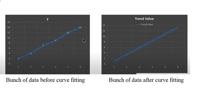

Objectives.1

Code for linear polynomial & cubic polynomial

• p(x)=ax+b where b are the real numbers. The highest degree of polynomial is ^1 means is known as linear polynomial.
• p(x)=a*x^3+b*x^2+c*x+d whera d is the real number. The highest degree of polynomial is ^3 means is known as cubic polynomial.

Program.1(linear polynomial)

clear all 
close all
clc
% preparing the data

given_data =load('given_data'); % insert the given_data by using load command 
temperature = given_data(:,1);  % All row of 1st coloumn data assigned as temperature
initial_cp = given_data(:,2);   % All row of 2nd coloumn data assigned as initial_cp

% curve fit
% cp =a*T+b
co_efficient =polyfit(temperature,initial_cp,1); % using polyfit command to find out the co_efficient value of (a,b,c,d) and the degree of polynomial is 1
predicted_cp_linear =polyval(co_efficient,temperature);% using polyfil command to find ou the prdiected_cp

% comparing the curvefit with original data
% plotting
hold on
plot(temperature,initial_cp,'linewidth',3,'color','r'); %plotting the temperature & initial_cp
plot(temperature,predicted_cp_linear,'LineWidth',3,'Color','b'); %plotting the temperature & predicted_cp_linear
xlabel('temperature [k]');
ylabel('initial & predicted cp [kj/kmol.k]');
title(' Linear Curve Fitting');
legend('old data','curve fit');

Program.2 (cubic polynomial)

clear all 
close all
clc
% preparing the data

given_data =load('given_data'); % insert the given_data by using load command 
temperature = given_data(:,1);  % All row of 1st coloumn data assigned as temperature
initial_cp = given_data(:,2);   % All row of 2nd coloumn data assigned as initial_cp

% curve fit

% cp =a*T^3+b*T^2*+c*T+d
co_efficient =polyfit(temperature,initial_cp,3); % using polyfit command to find out the co_efficient value of (a,b,c,d) and the degree of polynomial is 3
predicted_cp_cubic =polyval(co_efficient,temperature); % using polyfil command to find ou the prdiected_cp_cubic.

% For checking the goodness of fit
% Error= |y(i) - f(x(i))|
% Sum of the square due to error (SSE)
% R square
% SST= SSE+SSR
% Root mean squared error (RMSE) =sqrt(SSE/n)
n=3200;
error_cubic =initial_cp-predicted_cp_cubic;
SSE_cubic = sum(error_cubic).^2;
SSR_cubic = sum((predicted_cp_cubic-mean(initial_cp)).^2);
SST_cubic = SSR_cubic+SSE_cubic;
Rsquare_cubic =SSR_cubic/SST_cubic;


% comparing the curvefit with original data.
% plotting
hold on
plot(temperature,initial_cp,'linewidth',3,'color','r'); % plotting the temperature & initial_cp
plot(temperature,predicted_cp_cubic,'LineWidth',3,'Color','b');  %plotting the temperature & predicted_cp_cubic
xlabel('temperature [k]');
ylabel('cp [kj/kmol.k]');
title(' Cubic Curve Fitting');
legend('old data','curve fit');

Explanation

• clear all, close, all, clc commands are used.
• Insert the given data by using load command.
• The temperature and cp data is predpared by loading the original data set.
• Curve fit for coefficient and predicited cp is created using polyfit and polyval functions.

Polyfit - Polynomial curvefitting. This MATLABfunction returns the coefficient for a polynomial p(x) with respect to given input of degree of polynomial.

Polyval - Ploynomial evaluation. This MATLAB function evaluates polynomial p at each point in x and given the predicted cp which means new cp.

• The temperature vs cp data is plotted using original data set for linear polynomial and cubic polynomial.

• Hence the best fit for temperature and cp with degree (1 & 3) has been created using polyfit function and coefficient & temperature has been evaluated using polyval function
• Parameters used to measure the fitness characteristics are data set, its coefficient values, the order of polynomial equation
• The curve fit is plotted and compared with original data set.

OBJECTIVE 2:

Plotting of Linear and cubic polynomials:

The plots had been submitted below.

OBJECTIVE 3:

Splitwise method:

The process of splitting polynomial into 4 different parts to find best fit and perfect fit using the given parameters is called splitwise method.

clear all
close all
clc

% given_data
given_data =load('given_data'); %insert the given_data by using load command.
temperature =given_data(:,1);   % All row of 1st coloumn data assigned as temperature.
initial_cp =given_data(:,2);    % All row of 2nd coloumn data assigned as initial_cp.

% plotting
plot(temperature,initial_cp,'LineWidth',3,'Color','m');

% splitup the original data into 4 major parts.

% part =1
temperature1 =given_data(1:800,1); % split-up the first 800 rows of 1st coloumn and named as temperature1.
initial_cp1 =given_data(1:800,2);  % split-up the first 800 rows of 2nd coloumn and named as initial_cp1.

% part =2
temperature2 =given_data(801:1600,1); % split-up the second 800 rows of 1st coloumn and named as temperature2.
initial_cp2 =given_data(801:1600,2);  % split-up the second 800 rows of 2nd coloumn and named as initial_cp2.

% part =3
temperature3 =given_data(1601:2400,1); % split-up the third 800 rows of 1st coloumn and named as temperature3.
initial_cp3 =given_data(1601:2400,2);  % split-up the third 800 rows of 2nd coloumn and named as initial_cp3.

% part =4
temperature4 =given_data(2401:3200,1); % split-up the fourth 800 rows of 1st coloumn and named as temperature4.
initial_cp4 =given_data(2401:3200,2);  % split-up the fourth 800 rows of 2nd coloumn and named as initial_cp4.


% curvefit
% final_cp=a*t^2+b*t+c (degree of polynomial 2)

co_efficient1 =polyfit(temperature1,initial_cp1,2);% using polyfit command to find out the 1st 800 co_efficient value of (a,b,c) from the degree of polynomial is 2
final_cp1 =polyval(co_efficient1,temperature1); % using polyfil command to find out the 1st 800 of  the prdiected_cp
plot(temperature1,final_cp1,'linewidth',3,'Color','r');

co_efficient2 =polyfit(temperature2,initial_cp2,2); % using polyfit command to find out the 2nd 800 co_efficient value of (a,b,c) from the degree of polynomial is 2
final_cp2 =polyval(co_efficient2,temperature2); % using polyfil command to find out the 2nd 800 of  the prdiected_cp
plot(temperature2,final_cp2,'linewidth',3,'Color','b');

co_efficient3 =polyfit(temperature3,initial_cp3,2); % using polyfit command to find out the 3rd 800 co_efficient value of (a,b,c) from the degree of polynomial is 2
final_cp3 =polyval(co_efficient3,temperature3); % using polyfil command to find out the 3rd 800 of  the prdiected_cp
plot(temperature3,final_cp3,'linewidth',3,'Color','g');

co_efficient4 =polyfit(temperature4,initial_cp4,2); % using polyfit command to find out the 4th 800 co_efficient value of (a,b,c) from the degree of polynomial is 2
final_cp4 =polyval(co_efficient4,temperature4); % using polyfil command to find out the 4th 800 of  the prdiected_cp
plot(temperature4,final_cp4,'linewidth',3,'Color','y');

% joining of all splitted data & comparing the curvefit with original data

hold on
plot(temperature,initial_cp,'LineWidth',3,'Color','m');
plot(temperature1,final_cp1,'linewidth',3,'Color','r');
plot(temperature2,final_cp2,'linewidth',3,'Color','b');
plot(temperature3,final_cp3,'linewidth',3,'Color','g');
plot(temperature4,final_cp4,'linewidth',3,'Color','y');
xlabel('temperature [k]');
ylabel('initial & predicted cp [kj/kmol.k]');
title(' split-up Curve Fitting');
legend('predicted-cp4','initial-cp','predicted-cp1','predicted-cp2','predicted-cp3')

Stepwise Explanation for splitwise method:

• clear all, close all, clc command is used
• The temperature and cp data is predpared by loading the original data set.
• The original data set is divided into 4 parts, hence the temperature and cp is numbered and cp data is divided into 4 parts.
• Performing curvefit by splitting coefficient and predicited cp into 4 parts and using polyfit and polyval functions i have been find out the 4 parts value of co-efficient and final-cp.

OBJECTIVE 4:

Parameters used to measure fitness characteristics:

The parameters used to measure the curve fit are SSE and R-square.

• SSE: Sum of Squared Errors.

SSE=n∑i=1Error(i)2

• R-square

Increase the R-square to get bettter fit. if there is low R-square there is lousy fit (i.e) greater the SSE will give low R-square. Lesser the SSE gives Increased R-square. Maximum SSE = 0, maximum R-square = 1

It is calculated using'

R2=SSR/SST

here SSR = Sum of Square of Regression, it means the difference between the value of fitting function at a given point and arthemetic mean of data set.

If y=f(x) is the curve fit then SSR is defined as SSR=n∑i=1(f(x(i))−mean)2

If y=f(x) the SSE is defined as SSE=n∑i=1(y(i)−f(x(i)))2

hence, SST is calculated by summing SSR and SSE. SST=SSR+SSE and R2 can be calculated as R2=SSR/SST .