Parsing NASA thermodynamic data by using matlab

Aim: To read and calculate specific-heat,enthalpy,entropy from all the species from the given NASA thermodynamic data file.

Objectives:

1. To write a function that extracts the 14 co-efficients and calculates the specific-heat,enthalpy & entropy.
2. To plot the cp,entropy,enthalpy for the local temperature range of each species.
3. Saving the plots as images with approprite name and dump them in seperate folders for each species with suitable name.

Introdution:

Specific heat:

Specific heat, the quantity of heat required to raise the temperature of one gram of a substance by one Celsius degree. The units of specific heat are usually calories or joules per gram per Celsius degree. For example, the specific heat of water is 1 calorie (or 4.186 joules) per gram per Celsius degree.

% NASA Thermodynamic data and calculating the molecular weight
clear all
clear all
clc


% Opening the data from the folder
f1=fopen('thermo.txt','r');

% getting the header data
fgetl(f1);

% getting the global temp data
header_global_temp=fgetl(f1);

% split the global string data
A=strsplit(header_global_temp,' ');

% string data is converted into number and used for evaluation
global_low_temp=str2num(A{2});
global_mid_temp=str2num(A{3});
global_high_temp=str2num(A{4});

% Reading header theoritical data
for i=1:3
    fgetl(f1);
end

% reading all line data

for i=1:53
    tline1=fgetl(f1);
    tline2=fgetl(f1);
    tline3=fgetl(f1);
    tline4=fgetl(f1);

% Finding string for tline_2
loc_temp=strsplit(tline1,' ');
species_name=(loc_temp{1});
loc_low_temp=str2num(loc_temp{end-3});
loc_mid_temp=str2num(loc_temp{end-2});
loc_high_temp=str2num(loc_temp{end-1});


% finding the strings line 2
%  Finding the co_efficients
% finded string lines converted into numbers

a=findstr(tline2,'E');

a1=tline2(1:a(1)+3);
a1=str2num(a1);

a2=tline2(a(1)+4:a(2)+3);
a2=str2num(a2);

a3=tline2(a(2)+4:a(3)+3);
a3=str2num(a3);

a4=tline2(a(3)+4:a(4)+3);
a4=str2num(a4);

a5=tline2(a(4)+4:a(5)+3);
a5=str2num(a5);

% finding the strings line 3
%  Finding the co_efficients
% finded string lines converted into numbers
a=findstr(tline3,'E');

a6=tline3(1:a(1)+3);
a6=str2num(a6);

a7=tline3(a(1)+4:a(2)+3);
a7=str2num(a7);

a8=tline3(a(2)+4:a(3)+3);
a8=str2num(a8);

a9=tline3(a(3)+4:a(4)+3);
a9=str2num(a9);

a10=tline3(a(4)+4:a(5)+3);
a10=str2num(a10);

% finding the strings line 4
%  Finding the co_efficients
% finded string lines converted into numbers

a=strfind(tline4,"E");

a11=tline4(1:a(1)+3);
a11=str2num(a11);

a12=tline4(a(1)+4:a(2)+3);
a12=str2num(a12);

a13=tline4(a(2)+4:a(3)+3);
a13=str2num(a13);

a14=tline4(a(3)+4:a(4)+3);
a14=str2num(a14);

%  subsuite the values of a1 to a14 to calculate the enthalpy,entropy & specific_heat 
% Applying the universal gas constant
R=8.134;
T=linspace(loc_low_temp,loc_high_temp,300);

% calling the function's of cp,H,S
cp=specific_heat(a1,a2,a3,a4,a5,a6,a7,a8,a9,a10,R,T,loc_mid_temp);
H=enthalpy(a1,a2,a3,a4,a5,a6,a7,a8,a9,a10,a11,a12,T,loc_mid_temp,R);
S=entropy(a1,a2,a3,a4,a5,a6,a7,a8,a9,a10,a11,a12,a13,a14,R,T,loc_mid_temp);

    
% plotting
% creating a folder 'SPECIES' to save all the species_name
mkdir(['C:UsersgokulOneDriveDesktopskill-lyncchallengeschallenges outputchallenges outputfilrparsingnew',species_name]);

% plotting Cp vs T
figure(1);
plot(cp,T,'linewidth',3,'Color','r');
title('Specific-heat vs Temperature ');
xlabel('Specific-heat [j/k]');
ylabel('Temperature [k]');
saveas(1,'cp_vs_t.jpeg');

% plotting H vs T
figure(2);
plot(T,H,'linewidth',3,'Color','b');
title("Enthalpy vs Temperature");
xlabel('Enthalpy [j]');
ylabel('Temperature [k]');
saveas(2,'H_vs_T.jpeg');

% plotting S vs T
figure(3);
plot(S,T,'LineWidth',3,'Color','g');
title('Entropy vs Temperature');
xlabel('Entropy [kj-1/mol-1]');
ylabel('Temperature [k]');
saveas(3,'S_vs_T.jpeg');

cd(['C:UsersgokulOneDriveDesktopskill-lyncchallengeschallenges outputchallenges outputfilrparsingnew',species_name]);

% function calling to find molecular_weight
mole_weight=mol_weight(species_name);


end

clear all
clear all
clc

% Opening the data from the folder
f1=fopen('thermo.txt','r');

% getting the header data
fgetl(f1);

Explanation:

• Opening & reading the given data from the folder using fopen command.
• The command fopen is used to reading the thermodynamic data.
• The fgetl command is used to read the file and skip the file.

code:

% split the global string data
A=strsplit(header_global_temp,' ');

% string data is converted into number and used for evaluation
global_low_temp=str2num(A{2});

global_mid_temp=str2num(A{3});
global_high_temp=str2num(A{4});

Explanation: extract the global temperature

• The global temperature data can be stored in after header and also it is available in the form of 'string' type.
• using the command strsplit to get the string and it is stored in cell array.
• After that using the str2num command to convert the global temperature string format into number format.

code:

% Reading header theoritical data
for i=1:3
fgetl(f1);
end

Explanation: skipping the theoritical data

• After the extraction of global temperature next 3 line are theatorical data so we need to skip the file using for loop & getl command to skip the data.

Code:

for i=1:53
tline1=fgetl(f1);
tline2=fgetl(f1);
tline3=fgetl(f1);
tline4=fgetl(f1);

% Finding string for tline_2
loc_temp=strsplit(tline1,' ');
species_name=(loc_temp{1});
loc_low_temp=str2num(loc_temp{end-3});
loc_mid_temp=str2num(loc_temp{end-2});
loc_high_temp=str2num(loc_temp{end-1});

Explanation:Getting the temperature info from all species and make the co-efficient for that.

• After skipping the theoritical data by using getl command, a loop is created for 1:53 because we having 53 species in the given thermodynamic data.
• tline1=fgetl(f1) command is used to extract the 1st line of the all 53 species.
• tline2=fgetl(f1) command is used to extract the 2nd line of the all 53 species.
• tline3=fgetl(f1) command is used to extract the 3rd line of the all 53 species.
• tline4=fgetl(f1) command is used to extract the 4th line of the all 53 species.
• All species name and local temperature are available in tline1.so,using str2num command to change the string of local temp into number of local temp and the temp named as loc_low_temp,loc_med_temp,loc_high_temp.now tline job is completed,we have extract all the data from the 1st 53 lines species.

code:

% finding the strings line 2
% Finding the co_efficients
% finded string lines converted into numbers

a=findstr(tline2,'E');

a1=tline2(1:a(1)+3);
a1=str2num(a1);

a2=tline2(a(1)+4:a(2)+3);
a2=str2num(a2);

a3=tline2(a(2)+4:a(3)+3);
a3=str2num(a3);

a4=tline2(a(3)+4:a(4)+3);
a4=str2num(a4);

a5=tline2(a(4)+4:a(5)+3);
a5=str2num(a5);

% finding the strings line 3
% Finding the co_efficients
% finded string lines converted into numbers
a=findstr(tline3,'E');

a6=tline3(1:a(1)+3);
a6=str2num(a6);

a7=tline3(a(1)+4:a(2)+3);
a7=str2num(a7);

a8=tline3(a(2)+4:a(3)+3);
a8=str2num(a8);

a9=tline3(a(3)+4:a(4)+3);
a9=str2num(a9);

a10=tline3(a(4)+4:a(5)+3);
a10=str2num(a10);

% finding the strings line 4
% Finding the co_efficients
% finded string lines converted into numbers

a=strfind(tline4,"E");

a11=tline4(1:a(1)+3);
a11=str2num(a11);

a12=tline4(a(1)+4:a(2)+3);
a12=str2num(a12);

a13=tline4(a(2)+4:a(3)+3);
a13=str2num(a13);

a14=tline4(a(3)+4:a(4)+3);
a14=str2num(a14);

Explanation:Extracting the co-efficient values.

• Inorder to extract the co-efficient values,i got the lines by fgetl command and marked as line2,line3,line4 and i use this line to extract the co-efficient.
• In this case i'm using findstr(tline,'E) command is used to find the exponents E lies on the all given data.after finding of exponents E then extract into co-efficient using str2num command.this procedure is same as all 14 co efficient.
• For loop is used to find all three lines of co-efficients in a given data.

code

% subsuite the values of a1 to a14 to calculate the enthalpy,entropy & specific_heat
% Applying the universal gas constant
R=8.134;
T=linspace(loc_low_temp,loc_high_temp,300);

% calling the function's of cp,H,S
cp=specific_heat(a1,a2,a3,a4,a5,a6,a7,a8,a9,a10,R,T,loc_mid_temp);
H=enthalpy(a1,a2,a3,a4,a5,a6,a7,a8,a9,a10,a11,a12,T,loc_mid_temp,R);
S=entropy(a1,a2,a3,a4,a5,a6,a7,a8,a9,a10,a11,a12,a13,a14,R,T,loc_mid_temp);

Explanation:Calling the function for calculation

• In this case some of formula's are given to equitate with co-efficients and findout the values.The values are cp(specific heat),H(enthalpy),S(entropy).
• For loop is used for repeating these condition for all three at once cp,H&S
• if loop is used here because there a condition is applied for finding values of all 7 co-efficients of higher temperature and values of 7 co-efficient of lower temp.
• function codes can be mentioned below.

functiones codes

1.function to find specific heat:

function [cp]=specific_heat(a1,a2,a3,a4,a5,a6,a7,a8,a9,a10,R,T,loc_mid_temp);
if T>=loc_mid_temp
cp=(a1+a2.*(T)+a3.*(T.^2)+a4.*(T.^3)+a5.*(T.^4))*R;
else
[cp]=(a6+a7.*(T)+a8.*(T.^2)+a9.*(T.^3)+a10.*(T.^4))*R;
end
end

2.function to find enthalpy H

function H=enthalpy(a1,a2,a3,a4,a5,a6,a7,a8,a9,a10,a11,a12,T,loc_mid_temp,R)
if T>=loc_mid_temp
H=(a1*T+a2.*(T.^2)/2+a3.*(T.^3)/3+a4.*(T.^4)/4+a5.*(T.^5)/5+a6)*R
else
H=(a7*T+a8.*(T.^2)/2+a9.*(T.^3)/3+a10.*(T.^4)/4+a11.*(T.^5)/5+a12)*R
end
end

3.function to find entropy S

function [S]=entropy(a1,a2,a3,a4,a5,a6,a7,a8,a9,a10,a11,a12,a13,a14,R,T,loc_mid_temp)
if T>=loc_mid_temp
S=(a1.*log(T)+a2.*(T)+a3.*(T.^2)./2+a4.*(T.^3)./3+a5.*(T.^4)./4+a7)*R;
else
S=(a8.*log(T)+a9.*(T)+a10.*(T.^2)./2+a11.*(T.^3)./3+a12.*(T.^4)./4+a14)*R
end
end

objectives.2

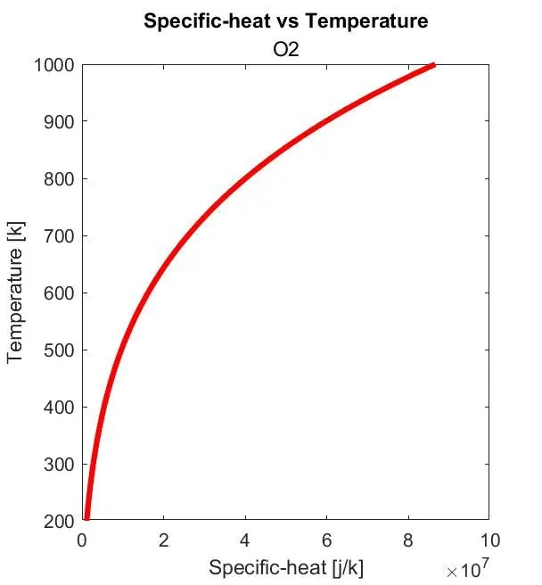
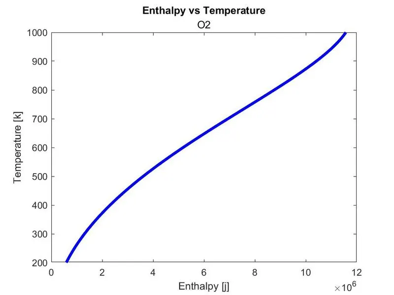
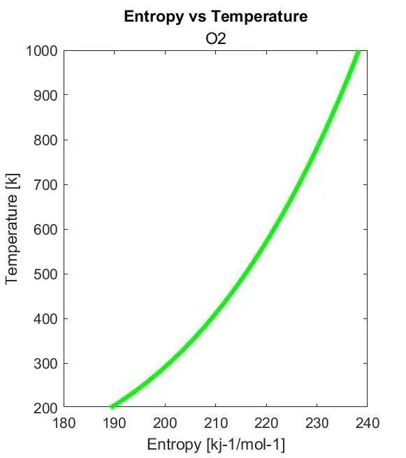
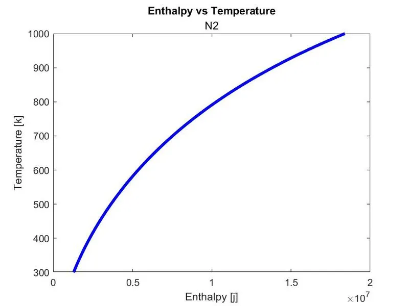
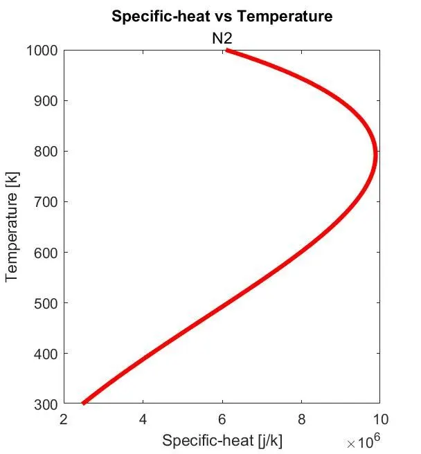
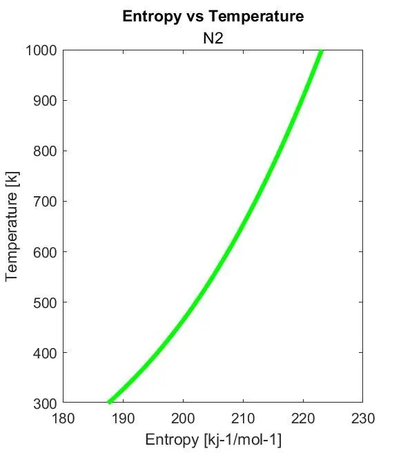
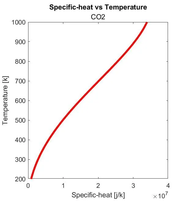
Plot the Cp, Enthalpy and Entropy for the local temperature range (low temperature : high temperature) specific for each species.

code:

% plotting Cp vs T
figure(1);
plot(cp,T,'linewidth',3,'Color','r');
title('Specific-heat vs Temperature ');
xlabel('Specific-heat [j/k]');
ylabel('Temperature [k]');
saveas(1,'cp_vs_t.jpeg');

% plotting H vs T
figure(2);
plot(T,H,'linewidth',3,'Color','b');
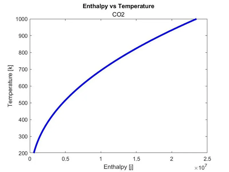
title("Enthalpy vs Temperature");
xlabel('Enthalpy [j]');
ylabel('Temperature [k]');
saveas(2,'H_vs_T.jpeg');

% plotting S vs T
figure(3);
plot(S,T,'LineWidth',3,'Color','g');
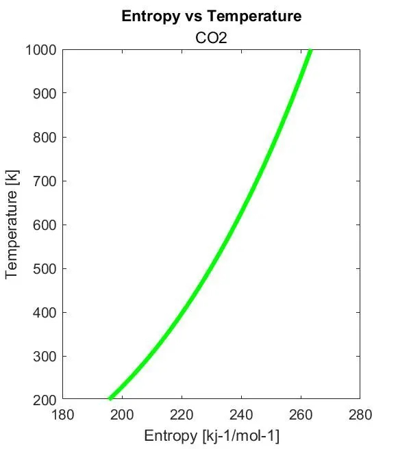
title('Entropy vs Temperature');
xlabel('Entropy [kj-1/mol-1]');
ylabel('Temperature [k]');
saveas(3,'S_vs_T.jpeg');

Explanation: plotting all the co-efficients.

• plot the graph between cp and temp,H vs temp,S vs temp.
• Titled the plot as specific-heat vs temperature using title command.
• x-label & y-label commands are used to naming the axis.
• saveas command is used to save the plots at an required format to the folder.

Objectives.3

Save the plots as images with appropriate names and dump them in separate folders for each species with suitable name. All these should be generated automatically and displays Screenshot of the window where all the folders are saved.

code:

mkdir(['C:UsersgokulOneDriveDesktopskill-lyncchallengeschallenges outputchallenges outputfilrparsingnew',species_name]);

Explanation:To creat a folder using matlab command

• mkdir command is used to create a folder,once we type the command then we go to the file manager and copy the link of the folder then then pasted on the matlab.
• cd command is used to define a path to the folder where the data has to be stored.

objectives.4

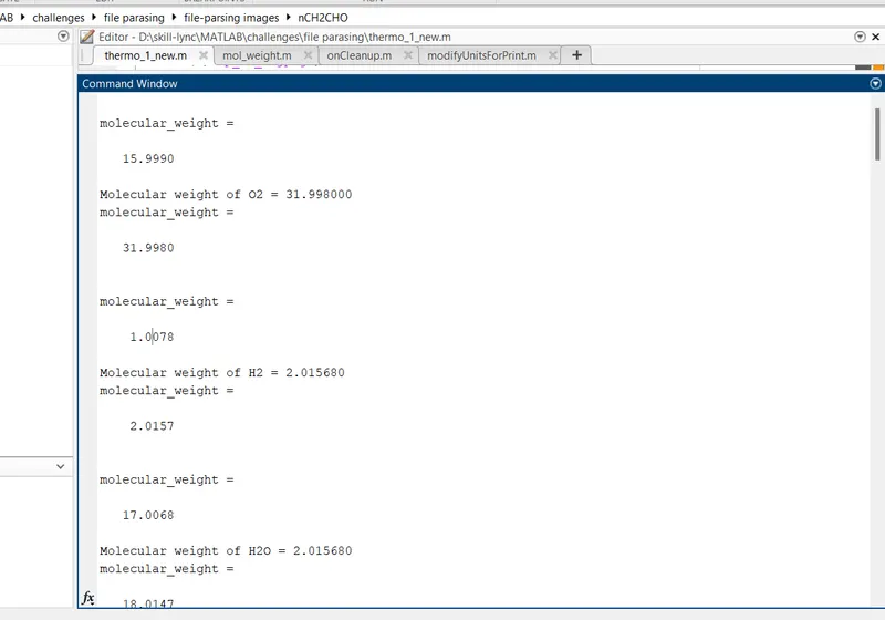
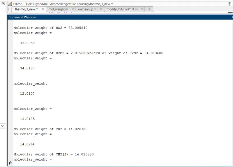
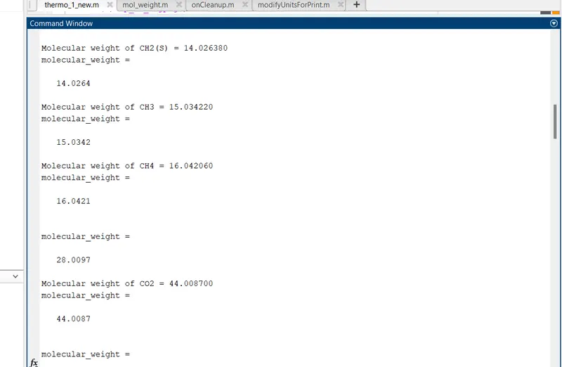
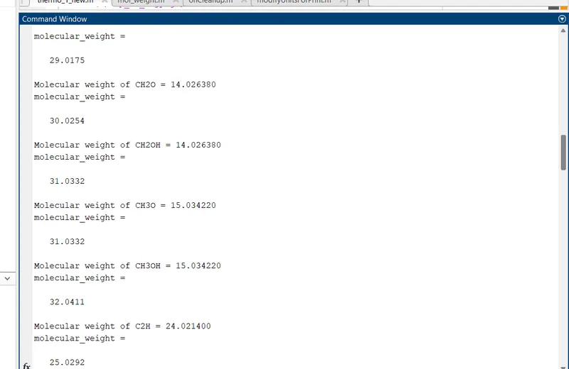
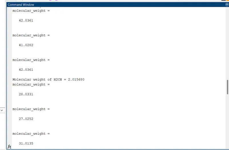
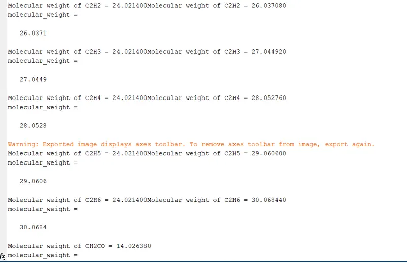
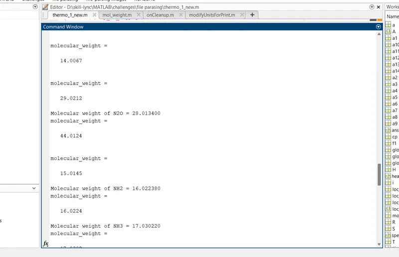
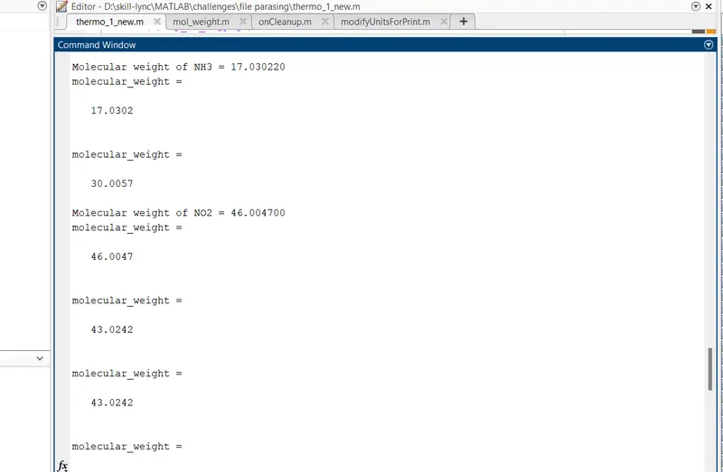
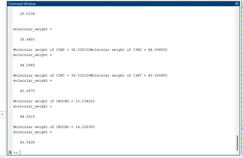
Calculate the molecular weight of each species and display it in the command window.

code

function [w]=mol_weight(species_name)
atomic_names=['H','C','O','N','A'];
atomic_weights=[1.00784,12.0107,15.999,14.0067,39.948];
w=0;

for i=1:length(species_name);
    for j=1:length(atomic_names);
        if strcmpi(species_name(i),atomic_names(j));
            w=w+atomic_weights(j);
            pos=j;
        end
        
        n=str2num(species_name(i));
    end

    if n>=1;

           w =w+atomic_weights(pos)*(n-1);
            k=fprintf('Molecular weight of %s = %f',species_name,w);
        end
    end

Explanation:

• A funnction is created to calculate the molecular weight of each species.then call the function in the main code to got the molecular weight for all species.
• Calculate the molecular weight of each species and display it in the command window are shown below.

fig for molcular values which displayed in the command window.

output:

• The attachement of all the folders saved in the windows are shown below
• Plots for o2, N2 and Co2 species

fig for dlsplaying the saved folder for each species.

Plots fig. for o2, N2 and Co2 species

1. Plots for o2 species:

2.Plots for N2 species:

3.Plots for Co2 species

Conclusion:

Using matlab the required data is read which is extracted from a given NASA thermodynamic data file and programmed to plot enthalpy,entropy&specific heat for all species.Molecular weight is calculated for all the species.