Week 4.1 - Genetic Algorithm
Aim
Write a program in Matlab to optimise the given stalagmite function
`f(x,y) = f_{1x} \times f_{2x} \times f_{1y} \times f_{2y}`
`f_{1x}= [sin(5.1\pi x +0.5)]^6`
Objective
- Write a code in MATLAB to optimise the stalagmite function and find the global maxima of the function.
- Clearly expalin the concept of genetic algorithm in your own words and also explain the syntax for ga in MATLAB in your report.
- Plot graphs for all 3 studies and for F maximum vs no. of iterations. Title and axes labels are a must, legends could be shown if necessary.
Solution
Optimization Using Genetic Algorithm
Optimization techniques are the techniques used to discover the best solution out of all the possible solutions available under the constraints present. The genetic algorithm is one such optimization algorithm built based on the natural evolutionary process of our nature. The algorithm repeatedly modifies a population of individual solutions. At each step, the genetic algorithm randomly selects individuals from the current population and uses them as parents to produce the children for the next generation. Over successive generations, the population "evolves" toward an optimal solution.
How GA works.
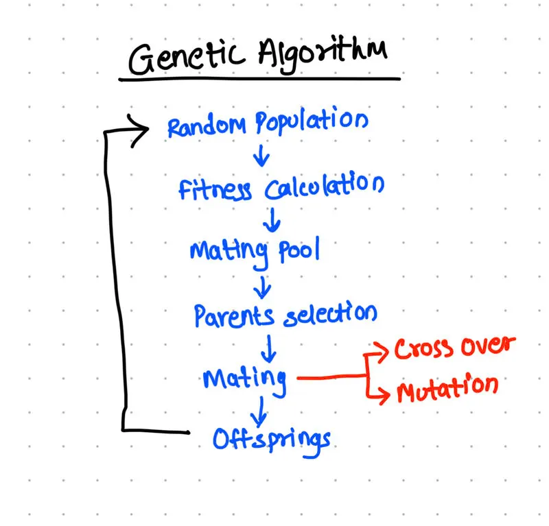
GA works on a population consisting a number of solution,
Each solution consists of some parameters that defines the solution. Also each solution has a fitness value associated to it. The result of the fitness function is the fitness value representing the quality of the solution. The higher the fitness value the higher the quality the solution.
Selection of the best individuals based on their quality is applied to generate a mating pool.
The individuals in the mating pool are called parents.
Every two parents selected from the mating pool will generate two offspring (children).
For every two parents selected, there are a number of variation operators to get applied such as:
1. Crossover (recombination): Crossover in GA generates new generation. By mutating the old generation parents, the new generation offspring comes by carrying genes from both parents. The amount of genes carried from each parent is random.
2. Mutation: For each offspring some genes are selected and its values are changed to generate mutation.
This process is repeated until a desired optimal or acceptable solution is found.
Matlab has an inbuilt function 'ga' that finds minimum of function using genetic algorithm.
For any given problem to optimize
function = f(x)
[x,fval] = ga(@function,nvar)
where fval = value of the fitness function at x nvar = number of design variables of the function.
Writing a code in MATLAB to optimise the stalagmite function and find the global maxima of the function
%stalagmite function

function [f] = stalagmite(input_vector)

x=input_vector(1);
y=input_vector(2);

f1_x = (sin(5.1*pi*x+0.5))^6;
f1_y = (sin(5.1*pi*y+0.5))^6;

f2_x = exp(-4*log(2)*((x-0.0667)^2/0.64));
f2_y = exp(-4*log(2)*((y-0.0667)^2/0.64));

f=-(f1_x*f2_x*f1_y*f2_y); %(-ve) sign is because we have to find maxima of the function

end
clear all
close all

clc

%Defining search space

x =linspace(0,0.6,150);
y =linspace(0,0.6,150);

%Creating a 2d Mesh

[xx,yy]=meshgrid(x,y);

%Evaluating the stalagmite function

for i=1:length(x)
	for j=1:length(y)

		input_vector(1)=xx(i,j);
		input_vector(2)=yy(i,j);
		func(i,j) = stalagmite(input_vector);

	end
end

[location,fval]=ga(@stalagmite,2)

surfc(xx,yy,func)
xlabel('x')
ylabel('y')
title('Stalagmite Function')
shading interp
Following plot was generated for our function.
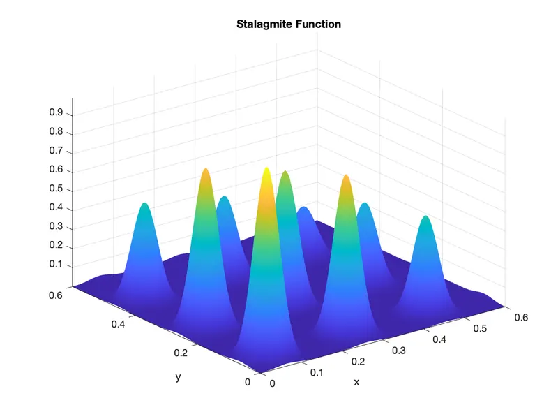
First Time when we run the program we get results as below
location =
23.3107 3.2442
fval =
0
Second time when we run the same program we get different results as shown
location =
32.9750 11.1953
fval =
0
Every time we run the program outputs a different result, this is because 'ga' function in in general uses random variables to determine the solution unless defines.
Writing Code to get optimum solution
To study statistical behavior of out code we have to modify our previous code as below
clear all
close all
clc

% Search Space

x=linspace(0,0.6,150);
y=linspace(0,0.6,150);

%Number of Iterations

iteration = 50;

%Creating a 2d Mesh

[xx,yy]=meshgrid(x,y);

%Evaluating the stalagmite function

for i=1:length(x)
	for j=1:length(y)

		input_vector(1)=xx(i,j);
		input_vector(2)=yy(i,j);

		func(i,j) = stalagmite(input_vector);

	end
end

%Study 1

tic

for i=1:iteration

	[input_vector,fopt(i)] = ga(@stalagmite,2);
	xopt(i)=input_vector(1);
	yopt(i)=input_vector(2);

end

study1_time = toc
subplot(2,1,1)
hold on
surfc(xx,yy,func)
shading interp
xlabel('X Value')
ylabel('Y Value')
plot3(xopt,yopt,fopt,'marker','o',MarkerSize=5,MarkerFaceColor='r')
subplot(2,1,2)
plot(fopt)
xlabel('Iteration')
ylabel('Maxima')
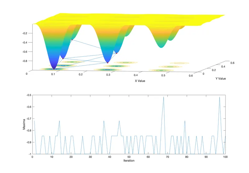
Following plot was generated for our function
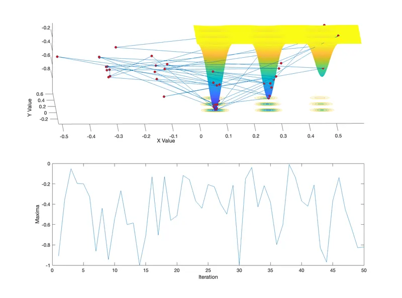
Upon observing we can see that the function is using random values (population) to optimize our results This is due to the 'ga' function in Matlab takes random values to minimize a function by default. Also it took 2.052 seconds to solve.
To Get more useful results we can define the search space for the function to select values from.
clear all
close all
clc

% Search Space

x=linspace(0,0.6,150);
y=linspace(0,0.6,150);

%Number of Iterations

iteration = 50; %Number of Iterations

%Defining lower and upper bounds

lb = [0,0];
ub = [1,1];

%Creating a 2d Mesh

[xx,yy]=meshgrid(x,y);

%Evaluating the stalagmite function

for i=1:length(x)
	for j=1:length(y)

		input_vector(1)=xx(i,j);
		input_vector(2)=yy(i,j);
		func(i,j) = stalagmite(input_vector);

	end
end

%Study 2

tic

for i=1:iteration
	[input_vector,fopt(i)] = ga(@stalagmite,2,[],[],[],[],lb,ub);
	xopt(i)=input_vector(1);
	yopt(i)=input_vector(2);
end

study2_time = toc

subplot(2,1,1)
hold on
surfc(xx,yy,func)
shading interp
xlabel('X Value')
ylabel('Y Value')
plot3(xopt,yopt,fopt,'marker','o',MarkerSize=5,MarkerFaceColor='r')
subplot(2,1,2)
plot(fopt)
xlabel('Iteration')
ylabel('Maxima')
Following plot was generated for our function
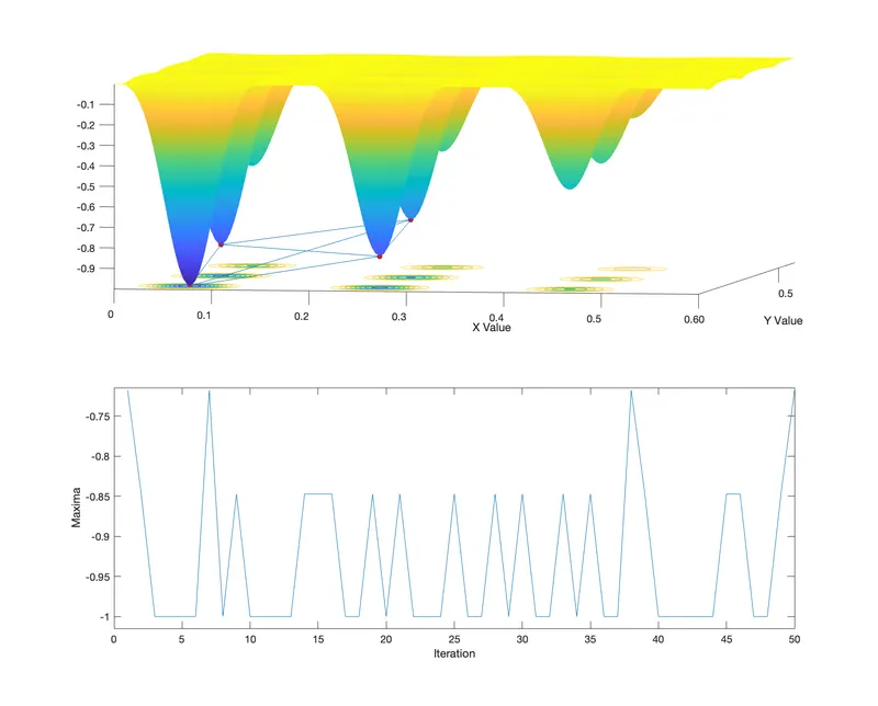
Upon observing we can see that the algorithm is using values from our defined function (stalagmite function) bounds to optimize our results. Still we not getting a maximum optimum value. Also, this time it took 3.2118 seconds to solve.
Increasing the number of iterations to further concise our results
Upon observing, we can see that even after increasing the number of iterations we are not getting useful result. Also, the time to solve increased from 3.2118 sec to 5.7309 sec without any satisfactory output.
clear all
close all
clc
% Search Space
x=linspace(0,0.6,150);
y=linspace(0,0.6,150);
%Number of Iterations
iteration = 50;
%Defining lower and upper bounds
lb = [0,0];
ub = [1,1];
%Creating a 2d Mesh
[xx,yy]=meshgrid(x,y);
%Evaluating the stalagmite function
for i=1:length(x)
for j=1:length(y)
input_vector(1)=xx(i,j);
input_vector(2)=yy(i,j);
func(i,j) = stalagmite(input_vector);
end
end
%Study 3
tic
%Defining population size
options=optimoptions('ga')
options=optimoptions(options,'PopulationSize',150);
for i=1:iteration
[input_vector,fopt(i)] = ga(@stalagmite,2,[],[],[],[],lb,ub,[],[],options);
xopt(i)=input_vector(1);
yopt(i)=input_vector(2);
end
study3_time = toc
subplot(2,1,1)
hold on
surfc(xx,yy,func)
shading interp
xlabel('X Value')
ylabel('Y Value')
plot3(xopt,yopt,fopt,'marker','o',MarkerSize=5,MarkerFaceColor='r')
subplot(2,1,2)
plot(fopt)
xlabel('Iteration')
ylabel('Maxima')
Following plot was generated for our function
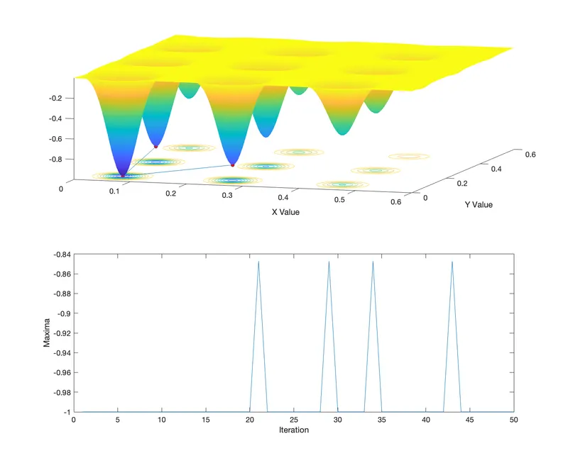
Upon observing, we can see that by defining population size to 150 (50 by default), we are getting close to the expected and predictable results, but in this case the time to solve the increased drastically from 3.2118 seconds to 782.6009 second.
To find optimal solution we can use a combination of no of iterations and population size to solve for maximum value with less time.
Following plot shows the best optimum solution with 50 iterations and 170 population size.
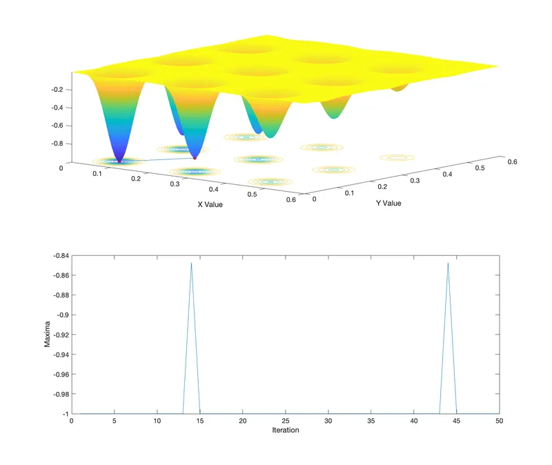
Step Wise Explanation of the code
Step 0
Writing Stalagmite function:
Writing the given function to find the maxima using ga.
%stalagmite function

function [f] = stalagmite(input_vector)

x=input_vector(1);
y=input_vector(2);

f1_x = (sin(5.1*pi*x+0.5))^6;
f1_y = (sin(5.1*pi*y+0.5))^6;

f2_x = exp(-4*log(2)*((x-0.0667)^2/0.64));
f2_y = exp(-4*log(2)*((y-0.0667)^2/0.64));

f=-(f1_x*f2_x*f1_y*f2_y); %(-ve) sign is because we have to find maxima of the function

end
Step 1
Initializing the Matlab:
These commands are used to clear the variables and plots stored in the memory from previous programs.
clear all
close all
clc
Step 2
Defining Inputs:
% Search Space

x=linspace(0,0.6,150);
y=linspace(0,0.6,150);

%Number of Iterations

iteration = 50;

%Defining lower and upper bounds

lb = [0,0];
ub = [1,1];
Step 3
Calculating stalagmite function:
%Creating a 2d Mesh

[xx,yy]=meshgrid(x,y);

%Evaluating the stalagmite function

for i=1:length(x)

	for j=1:length(y)

		input_vector(1)=xx(i,j);
		input_vector(2)=yy(i,j);
		func(i,j) = stalagmite(input_vector);

	end

end
Step 4
Coding optimization using ga:
%Study 3

tic
%Defining population size

options=optimoptions('ga')
options=optimoptions(options,'PopulationSize',150);


for i=1:iteration

	[input_vector,fopt(i)] = ga(@stalagmite,2,[],[],[],[],lb,ub,[],[],options);
	xopt(i)=input_vector(1);
	yopt(i)=input_vector(2);

end

study3_time = toc
Step 5
Plotting:
subplot(2,1,1)
hold on
surfc(xx,yy,func)
shading interp
xlabel('X Value')
ylabel('Y Value')
plot3(xopt,yopt,fopt,'marker','o',MarkerSize=5,MarkerFaceColor='r')
subplot(2,1,2)
plot(fopt)
xlabel('Iteration')
ylabel('Maxima')
Errors
1. Unrecognized function or variable 'x'.
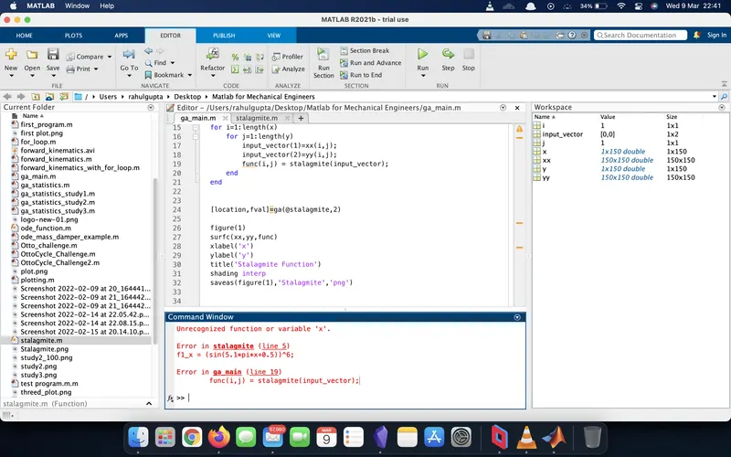
solved by defining x and y variables in function itself.