Week 3 - Solving second order ODEs
Aim
Write a program in Matlab\Octave that will simulate the pendulum motion.
Objective
-
Write a program that solves the following ODE This ODE represents the equation of motion of a simple pendulum with damping
In the above equation, g = gravity in m/s2,
L = length of the pendulum in m,
m = mass of the ball in kg,
b=damping coefficient.
-
To animate the motion of the pendulum.
Solution
Representation Diagram:
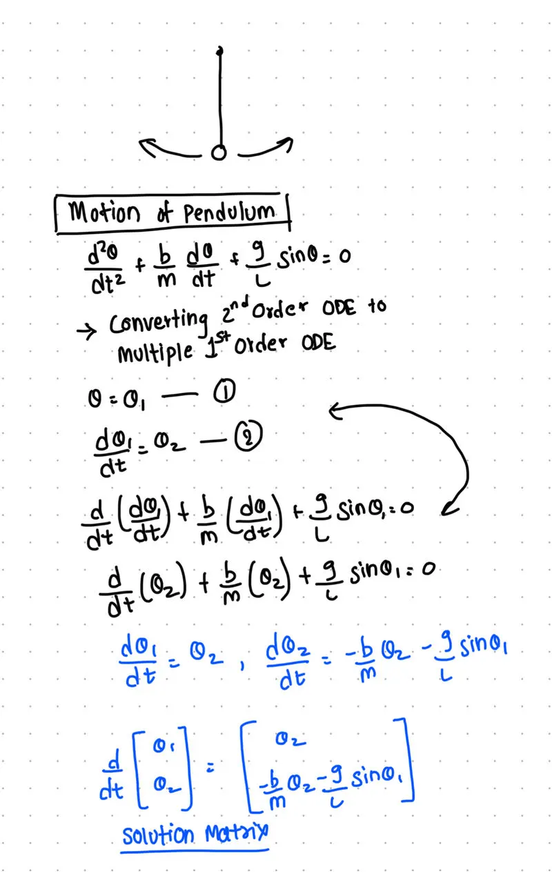
The Given equation of motion of pendulum is a second order ODE, hence we need to simplify the given equation into multiples of first order ODE, which further can be solved using Matlab's inbuilt ODE solver.
The given equation can be simplified into
$$\frac{d\theta_{1}}{dt} = \theta_{2}$$
$$\frac{d\theta_{2}}{dt} = -\frac{b}{m}\theta_{2}-\frac{g}{l}sin\theta_{1}$$
The Solution matrix is given as
$$\frac{d}{dt}\begin{bmatrix}
\theta_{1}\\
\theta_{2}
\end{bmatrix}= \begin{bmatrix}\theta_{2}\\-\frac{b}{m}\theta_2 \left( -\frac{g}{l}sin\theta_{2} \right) \\ \end{bmatrix} $$
Writing a function in Matlab to solve this ODE
% function [variable to store output] = 'Function name(time,angular displacement,damping coeff.,gravity,length of string,mass)'
function [dtheta_dt] = ode_function(t,theta,b,g,l,m)

  theta1=theta(1)
  theta2=theta(2)
  dtheta1_dt=theta2;
  dtheta2_dt=-b/m*theta2*((-g/l)*theta1);

  [dtheta_dt]=[dtheta1_dt; dtheta2_dt]
end
We can call this function in our main program to solve for motion of pendulum.
Writing a program to plot time value graph of the behavior or our pendulum.
clear all
close all
clc


%Defining Initial condition to solve for ODE

theta_0= [0;3] %Initially at t=0 angular displacement is zero and angular velocity is 3,

t_span= linspace(0,20,500) %to solve from 0 to 20 sec with 500 values inbetween 0 to 20.

%Calling our pendulum function

%[matrix to store results] = name of the function(@(function of variables) function name(values),time range,initial condition)

[t,result]= ode45(@(t,theta) ode_function(t,theta,0.05,9.81,1,1),t_span,theta_0)

angular_displacement= result(:,1); %storing result 1
angular_velocity = result(:,2); %storing result 2

subplot(2,1,1)

plot(t,angular_displacement,LineWidth=1,Color='r')
title('Angular DIsplacement WRT Time')
ylim([-4 4])
xlabel('Time')
ylabel('Displacement')

subplot(2,1,2)

plot(t,angular_velocity,LineWidth=1,Color='b')
title('Angular Velocity WRT Time')
ylim([-4 4])
xlabel('Time')
ylabel('Velocity')
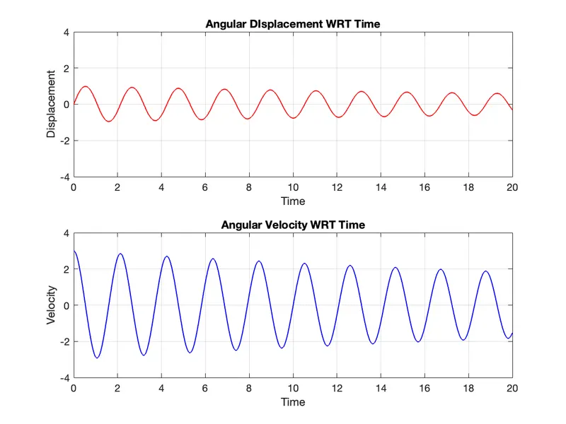
Following Graph was generated after the solution for angular displacement and velocity wrt. time.
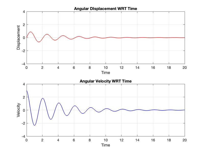
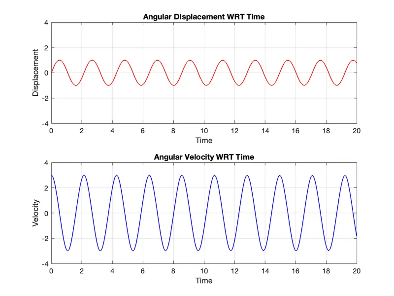
To verify if my code was correct i changed the value of damping coefficient to check if it behaves as expected.
If we increase or decrease the damping coefficient the displacement and velocity should change accordingly and generate graphs respectively.
1. For b=0.5 (Higher Damping Coeff. results in )
2. For b=0 (Lower Damping Coeff. results in )
Modifying our program to simulate the motion of pendulum.
Representation Diagram:
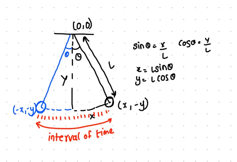
To Simulate the motion of pendulum we need two points. Since top end of the pendulum is fixed, we need to find the position of second point, i.e. the position of the mass of pendulum at every interval of time.
clear all
close all
clc


%Defining Initial condition to solve for ODE

theta_0= [0;3] %Initially at t=0 angular displacement is zero and angular velocity is 3,

t_span= linspace(0,20,500) %to solve from 0 to 20 sec with 10 values inbetween 0 to 20.

%Calling our pendulum function

%[matrix to store results] = (name of the function(@(function of variables)),function name(values),time range,initial condition)

[t,result]= ode45(@(t,theta) ode_function(t,theta,0.05,9.81,1,1),t_span,theta_0)

angular_displacement= result(:,1);

angular_velocity = result(:,2);

%{

subplot(2,1,1)
plot(t,angular_displacement,LineWidth=1,Color='r')
title('Angular DIsplacement WRT Time')
ylim([-4 4])
xlabel('Time')
ylabel('Displacement')
grid on

subplot(2,1,2)
plot(t,angular_velocity,LineWidth=1,Color='b')
title('Angular Velocity WRT Time')
ylim([-4 4])
xlabel('Time')
ylabel('Velocity')
grid on

%}

%To Simulate Motion of Pendulum

x0=0
y0=0

ct=1 %Counter To save frame
l=1 %Length

for i=1:length(t_span)

x1=l*sin(angular_displacement(i));

y1=-l*cos(angular_displacement(i));

plot([x0 x1],[y0 y1],[x1 x1],[y1 y1],'o','MarkerSize',40,'LineWidth',1)
axis([-1.2 1.2 -1.5 0.5])

pause(0.1)
grid on

M(ct)=getframe(gcf);
ct=ct+1;

end

%Generate Video File

movie(M)
videofile=VideoWriter('Motion of Pendulum','Uncompressed AVI');
open(videofile)
writeVideo(videofile,M)
close(videofile)
Following Video Output is generated.
https://drive.google.com/file/d/1z_olnZVISef37bV1Iqnv4myZp9CYGOeF/view?usp=sharing
Explanation of the code
Step 0
Writing a Matlab function to solve for motion of pendulum. This function will be called in our main function to plot various graphs.
% function [variable to store output] = 'Function name(time,angular displacement,damping coeff.,gravity,length of string,mass)'

function [dtheta_dt] = ode_function(t,theta,b,g,l,m)

theta1=theta(1)
theta2=theta(2)
dtheta1_dt=theta2;
dtheta2_dt=-b/m*theta2-(g/l)*sin(theta1);

[dtheta_dt]=[dtheta1_dt; dtheta2_dt]

end
Step 1
Initializing the Matlab:
These commands are used to clear the variables and plots stored in the memory from previous programs.
clear all
close all
clc
Step 2
Defining Initial Conditions:
To solve ODE We need to define initial conditions and time span for which the equation will be solved. This Initial condition value and time span value will be used by matlab's 'ode45' solver to solve the equation.
%Defining Initial condition to solve for ODE

theta_0= [0;3] %Initially at t=0 angular displacement is zero and angular velocity is 3,

t_span= linspace(0,20,500) %to solve from 0 to 20 sec with 10 values inbetween 0 to 20.
Step 3
Calling Our Pendulum Equation Solver Function:
The Pendulum Solving Function we had written in step 0, is called to solve for the motion of the pendulum and store the result vectors in the variables as mentioned.
%Calling our pendulum function

%[matrix to store results] = (name of the function(@(function of variables)),function name(values),time range,initial condition)

[t,result]= ode45(@(t,theta) ode_function(t,theta,0.05,9.81,1,1),t_span,theta_0)

angular_displacement= result(:,1);

angular_velocity = result(:,2);
Step 4
Plotting The Results :
subplot(2,1,1)
plot(t,angular_displacement,LineWidth=1,Color='r')

title('Angular DIsplacement WRT Time')
ylim([-4 4])
xlabel('Time')
ylabel('Displacement')
grid on

subplot(2,1,2)
plot(t,angular_velocity,LineWidth=1,Color='b')
title('Angular Velocity WRT Time')
ylim([-4 4])
xlabel('Time')
ylabel('Velocity')
grid on
Following plot was generated.
Step 5
Simulating the motion of pendulum:
x0=0
y0=0
ct=1
l=1

for i=1:length(t_span)
x1=l*sin(angular_displacement(i));
y1=-l*cos(angular_displacement(i));
plot([x0 x1],[y0 y1],[x1 x1],[y1 y1],'o','MarkerSize',40,'LineWidth',1)

axis([-1.2 1.2 -1.5 0.5])
pause(0.1)

grid on

M(ct)=getframe(gcf);
ct=ct+1;

end
Step 6
Generating Video File:
%Generate Video File

movie(M)
videofile=VideoWriter('Motion of Pendulum','Uncompressed AVI');
open(videofile)
writeVideo(videofile,M)
close(videofile)
Errors
1. Invalid Expression
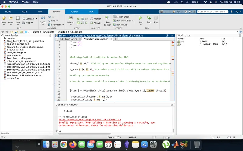
Solved by removing ',' after ode45(@(t,theta)-' statement.
2. mismatched delimiters
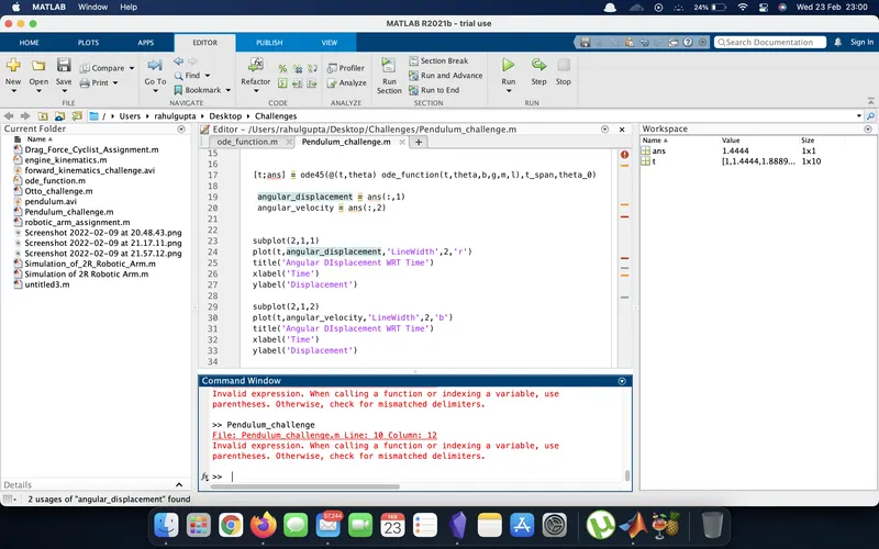
solved by storing results in a column vector. [t,ans] to [t;ans].
3. Invalid Expression (Forgot to put linspace in t_range)
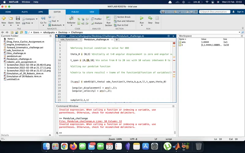
Solved by adding 'linspace' after tspan = ...
4.Error using odearguments (line 93) @(T,THETA)ODE_FUNCTION(T,THETA,0.05,9.81,1,1) must return a column vector.
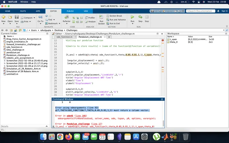
Solved by adding ';' in '[dtheta_dt]=[dtheta1_dt dtheta2_dt]' results of the function code.