Project 2 - Rankine cycle Simulator
Aim
Write a Code in octave to simulate Rankine Cycle.
Objective
- Create a Rankine Cycle Simulator using OCTAVE/MATLAB.
- Calculate the state points of the Rankine Cycle (any type of your choice) based on user inputs.
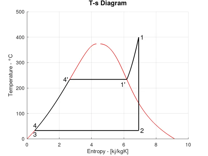
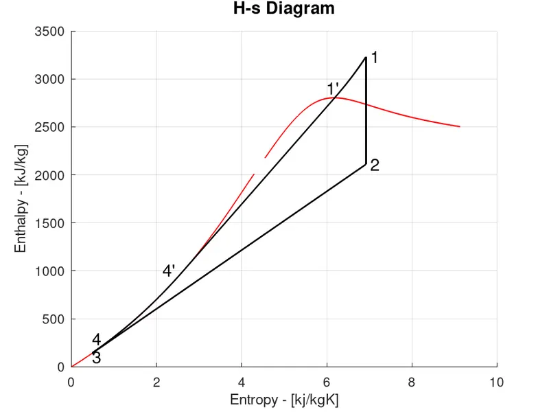
- Plot the corresponding T-s and h-s plots for the given set of inputs.
Solution
Theory
The Rankine cycle is an idealized thermodynamic cycle describing the process by which certain heat engines, such as steam turbines or reciprocating steam engines, allow mechanical work to be extracted from a fluid as it moves between a heat source and heat sink Heat energy is supplied to the system via a boiler where the working fluid (typically water) is converted to a high pressure gaseous state (steam) in order to turn a turbine. After passing over the turbine the fluid is allowed to condense back into a liquid state as waste heat energy is rejected before being returned to boiler, completing the cycle.
For each process in the vapour power cycle, it is possible to assume a hypothetical or ideal process which represents the basic intended operation.
For the steam boiler, this would be a reversible constant pressure heating process of water to form steam, for the turbine the ideal process would be a reversible adiabatic expansion of steam, for the condenser it would be a reversible constant pressure heat rejection as the steam condenses till it becomes saturated liquid, and for the pump, the ideal process would be the reversible adiabatic compression of this liquid ending at the initial pressure.
Figure shows the flow diagram of the Rankine cycle.
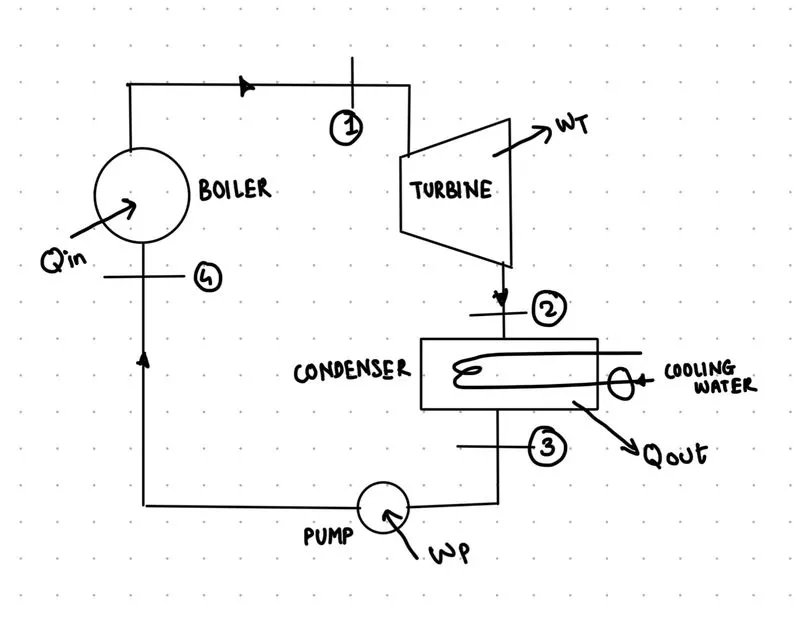
For any given pressure, the steam approaching the turbine may be dry saturated (state 1) wet (state 1'), or super-heated (state 1"), but the fluid approaching the pump is, in each case, saturated liquid (state 3). Steam expands reversibly and adiabiatically in the turbine from state 1 to state 2 (or 1' to 2', or 1" to 2"), the steam leaving the turbine condenses to water in the condenser reversibly at constant pressure from state 2 (or 2', or 2") to state 3, the water at state 3 is then pumped to the boiler at state 4 reversibly and adiabatically, and the water is heated in the boiler to form steam reversibly at constant pressure from state 4 to state 1 (or 1' or 1").
- 1 - 2 is Isentropic Expansion in the Turbine
- 2 - 3 is Constant Pressure Heat Rejection by the Condenser
- 3 - 4 is Isentropic Compression in the Pump
- 4 - 1 is Constant Pressure Heat Addition by the Boiler
`$${\dot {Q}} - \text{Heat Flow Rate}$$`
`$${\dot {m}} - \text{Mass Flow Rate}$$`
`$${{W}} - \text{Mechanical Power}$$`
`$${\eta_{cycle} - \text{Thermodynamic Efficiency of the Process}}$$`
`$${\displaystyle h_{1},h_{2},h_{3},h_{4}} - \text{Specific Enthalpies at Indicated Points}$$`
`$${\displaystyle p_{1},p_{2}} - \text{Pressures Before and After the Compression Process }$$`
For the given cycle
`$$\sum_{cycle}^{} Q_{net} = \sum_{cycle}^{} W_{net}$$`
`$$Q_{1} - Q_{2} = W_{turbine} - W_{pump}$$`
`$$Q_{1} = \text{heat transferred to the working fluid (kJ/kg)}$$`
`$$Q_{2} = \text{heat rejected from the working fluid (kJ/kg)}$$`
`$$W_{turbine} = \text{work transferred from the working fluid (kJ/kg)}$$`
`$$W_{pump} = \text{work transferred into the working fluid (kJ/kg)}$$`
Applying the steady flow energy equation to each of the processes on the basis of unit mass of fluid, and neglecting changes in kinetic and potential energy, the work and heat quantities can be evaluated in terms of the properties of the fluid.
For 1 kg fluid
The S.F.E.E. for the boiler is given as
`$$h_{4} + Q_{1} = h_{1}$$`
`$$\therefore Q_{1} = h_{1} - h_{4}$$`
The S.F.E.E. for the turbine is given as
`$$h_{1} = W_{turbine} + h_{2}$$`
`$$\therefore W_{turbine} = h_{1} - h_{2}$$`
Similarly. the S.F.E.E. for the condenser is
`$$h_{2} = Q_{2} + h_{3}$$`
`$$\therefore Q_{2} = h_{2} - h_{3}$$`
and the S.F.E.E. for the pump is
`$$h_{3} + W_{pump} = h_{4}$$`
`$$\therefore W_{pump} = h_{4} - h_{3}$$`
The Efficiency of the cycle is given as
`$$\eta_{cycle} = \frac{W_{net}}{Q_{1}} = \frac{W_{turbine} - W_{pump}}{Q_{1}} = \frac{Q_{1} - Q_{2}}{Q_{1}} = 1-\frac{Q_{2}}{Q_{1}}$$`
Back work ratio is defined as the ratio between the work done by the compressor to the work done by turbine.
`$$\therefore \text {Back Work Ratio} = \frac{W_{pump}}{W_{turbine}}$$`
The capacity of a steam plant is often expressed in terms of steam rate, which is defined as the rate of steam flow (kg/h) required to produce unit shaft output (1 kW).
`$$\therefore \text {Specific Steam Consumption} = \frac{3600}{W_{turbine}-W_{pump}}$$`
Writing a program in octave to solve the Rankine cycle for given input.
clear all;
close all;
clc;

%% Title
disp('')
fprintf('RANKINE CYCLE SIMULATOR')
disp('')

fprintf('\n 1 - 2 is Isentropic Expansion in the Turbine ')
fprintf('\n 2 - 3 is Constant Pressure Heat Rejection by the Condenser ')
fprintf('\n 3 - 4 is Isentropic Compression in the Pump')
printf('\n 4 - 1 is Constant Pressure Heat Addition by the Boiler')

disp('')
disp('')

%%Input

p1=input('Enter the Pressure at Turbine Inlet (in Bar):');
t1=input('Enter the Temperature at Turbine Inlet (in Degree Celcius):');
p2=input('Enter the Pressure at Condenser (in Bar):');


ts_p1=XSteam('Tsat_p',p1); %saturation temperature
hf_p1=XSteam('hL_p',p1);
hfg_p1=XSteam('h_pT',p1,t1);
hg_p1=XSteam('hV_p',p1);
sf_p1=XSteam('sL_p',p1);
sfg_p1=XSteam('s_pT',p1,t1);
sg_p1=XSteam('sV_p',p1);

ts_p2=XSteam('Tsat_p',p2); %saturation temperature
hf_p2=XSteam('hL_p',p2);
hg_p2=XSteam('hV_p',p2);
sf_p2=XSteam('sL_p',p2);
sg_p2=XSteam('sV_p',p2);

%%State Point 1 (Turbine Inlet)

h1=hfg_p1;
s1=sfg_p1;

fprintf('\nAt State Point 1:')
fprintf('\n  P1 is : %.2f Bar',p1)
fprintf('\n  T1 is : %.2f Degree Celsius',t1)
fprintf('\n  H1 is : %.2f kJ/kg',h1)
fprintf('\n  S1 is : %.2f kJ/kgK',s1)

%%State Point 2 (Condenser Inlet)

s2=s1; % 1-2 Isentropic Expansion
x2=(s2-sf_p2)/(sg_p2-sf_p2);
h2=hf_p2+x2*(hg_p2 - hf_p2);
t2=XSteam('T_hs',h2,s2);

disp('')
fprintf('\nAt State Point 2:')
fprintf('\n  P2 is : %.2f Bar',p2)
fprintf('\n  T2 is : %.2f Degree Celsius',t2)
fprintf('\n  H2 is : %.2f kJ/kg',h2)
fprintf('\n  S2 is : %.2f kJ/kgK',s2)
fprintf('\n  X2 is : %.2f',x2)


%%State Point 3 (Pump Inlet)
p3 = p2; %2 - 3 is Constant Pressure Heat Rejection by the Condenser
h3=XSteam('hL_p',p3);
s3=XSteam('sL_p',p3);
t3=XSteam('T_hs',h3,s3);

disp('')
fprintf('\nAt State Point 3:')
fprintf('\n  P3 is : %.2f Bar',p3)
fprintf('\n  T3 is : %.2f Degree Celsius',t3)
fprintf('\n  H3 is : %.2f kJ/kg',h3)
fprintf('\n  S3 is : %.2f kJ/kgK',s3)


%%State Point 4 (boiler inlet)
s4=s3; %3 - 4 is Isentropic Compression in the Pump
p4=p1;

h4=XSteam('h_ps',p4,s4);
t4=XSteam('T_hs',h4,s4);

disp('')
fprintf('\nAt State Point 4:')
fprintf('\n  P4 is : %.2f Bar',p4)
fprintf('\n  T4 is : %.2f Degree Celsius',t4)
fprintf('\n  H4 is : %.2f kJ/kg',h4)
fprintf('\n  S4 is : %.2f kJ/kgK',s4)

%Turbine Work
w_turbine = h1-h2;

%Pump Work
w_pump=h4-h3;

%Net Work
w_net=w_turbine-w_pump;

q_in=h1-h4;
q_out=h2-h3;

%Thermal Efficiency
thermal_efficiency=(w_net/q_in)*100;

%Back work ratio
bwr=w_pump/w_turbine;

%Specific Steam Consumption
ssc=3600/(w_net);

disp('')
fprintf('\n  Wt is : %.2f kJ/kg',w_turbine)
fprintf('\n  Wp is : %.2f kJ/kg',w_pump)
fprintf('\n  Wnet is : %.2f kJ/kg',w_net)
fprintf('\n  Ntherm is : %.2f Percent',thermal_efficiency)
fprintf('\n  S.S.C is : %.2f kg/kWh',ssc)
fprintf('\n  BWR is : %.5f',bwr)


%%Plotting T-s diagram

t=linspace(1,t1+100,1000);

ts4=XSteam('Tsat_p',p4);
sl_ts4=XSteam('sL_T',ts4);
sv_ts4=XSteam('sV_T',ts4);

for i=1:length(t)
  sl(i)=XSteam('sL_T',t(i));
  sv(i)=XSteam('sV_T',t(i));
  hl(i)=XSteam('hL_T',t(i));
  hv(i)=XSteam('hV_T',t(i));
end


s_1=linspace(sg_p1,s1,100);

for k=1:length(s_1)
  t11(k)=XSteam('T_ps',p1,s_1(k));
end

s_4=linspace(s4,sg_p1,100);
for l=1:length(s_4)
  t44(l)=XSteam('T_ps',p1,s_4(l));
end

figure(1)
hold on
grid on
title('T-s Diagram','fontsize',13)
plot(sl,t,'linewidth',1,'color','r')
plot(sv,t,'linewidth',1,'color','r')
plot([s1,s2],[t1,t2],'linewidth',1.5,'color','k')
plot([s2,s3],[t2,t3],'linewidth',1.5,'color','k')
plot([s3,s4],[t3,t4],'linewidth',1.5,'color','k')
plot(s_4,t44,'linewidth',1.5,'color','k')
plot(s_1,t11,'linewidth',1.5,'color','k')

xlabel('Entropy - [kj/kgK]')
ylabel('Temperature - \degC')

text(s1+0.1,t1,'1','fontsize',13)
text(s2+0.1,t2,'2','fontsize',13)
text(s3-0.1,t3-15,'3','fontsize',13)
text(s4-0.1,t4+20,'4','fontsize',13)
text(sg_p1-0.4,ts_p1-20,'1''','fontsize',13)
text(sf_p1-0.4,ts_p1,'4''','fontsize',13)
saveas(1,'Temperature Entropy Diagram','png')
hold off


%%Plotting H-s diagram


h_1=linspace(hg_p1,h1,100);

for m=1:length(h_1)
  s11(m)=XSteam('s_ph',p1,h_1(m));
end

h_4=linspace(hg_p1,h4,100);
for n=1:length(s_4)
  s44(n)=XSteam('s_ph',p1,h_4(n));
end

figure(2)

hold on
grid on
title('H-s Diagram','fontsize',13)
plot(sl,hl,'linewidth',1,'color','r')
plot(sv,hv,'linewidth',1,'color','r')
plot([s1,s2],[h1,h2],'linewidth',1.5,'color','k')
plot([s2,s3],[h2,h3],'linewidth',1.5,'color','k')
plot([s3,s4],[h3,h4],'linewidth',1.5,'color','k')
plot(s11,h_1,'linewidth',1.5,'color','k')
plot(s44,h_4,'linewidth',1.5,'color','k')

xlabel('Entropy - [kj/kgK]')
ylabel('Enthalpy - [kJ/kg]')

text(s1+0.1,h1,'1','fontsize',13)
text(s2+0.1,h2,'2','fontsize',13)
text(s3,h3-40,'3','fontsize',13)
text(s4,h4+150,'4','fontsize',13)
text(sf_p1-0.5,hf_p1,'4''','fontsize',13)
text(sg_p1-0.2,hg_p1+100,'1''','fontsize',13)
saveas(2,'Enthalpy Entropy Diagram','png')
hold off
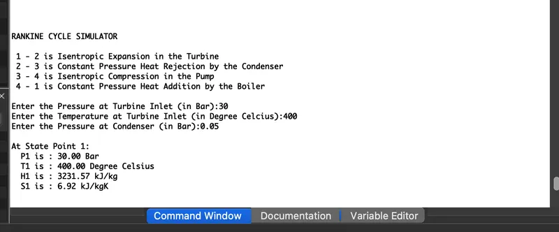
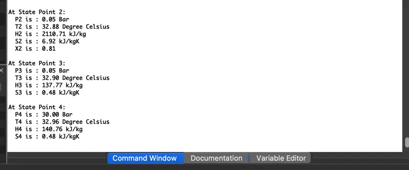
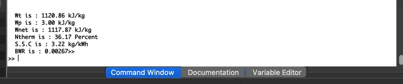
The above code takes input from the user and calculates the required parameters at every state point to plot the T-s Diagram and H-s Diagram respectively as given below.
Step Wise Explanation of the code
Step 0
Initializing the octave:
These commands are used to clear the variables and plots stored in the memory from previous programs.
clear all
close all
clc
Step 1
Display Title and accepting user input and finding Water and steam properties from 'Xsteam Library' at given pressure p1 and p2:
%% Title
disp('')
fprintf('RANKINE CYCLE SIMULATOR')
disp('')

fprintf('\n 1 - 2 is Isentropic Expansion in the Turbine ')
fprintf('\n 2 - 3 is Constant Pressure Heat Rejection by the Condenser ')
fprintf('\n 3 - 4 is Isentropic Compression in the Pump')
printf('\n 4 - 1 is Constant Pressure Heat Addition by the Boiler')

disp('')
disp('')

%%Input

p1=input('Enter the Pressure at Turbine Inlet (in Bar):');
t1=input('Enter the Temperature at Turbine Inlet (in Degree Celcius):');
p2=input('Enter the Pressure at Condenser (in Bar):');


ts_p1=XSteam('Tsat_p',p1); %saturation temperature
hf_p1=XSteam('hL_p',p1);
hfg_p1=XSteam('h_pT',p1,t1);
hg_p1=XSteam('hV_p',p1);
sf_p1=XSteam('sL_p',p1);
sfg_p1=XSteam('s_pT',p1,t1);
sg_p1=XSteam('sV_p',p1);

ts_p2=XSteam('Tsat_p',p2); %saturation temperature
hf_p2=XSteam('hL_p',p2);
hg_p2=XSteam('hV_p',p2);
sf_p2=XSteam('sL_p',p2);
sg_p2=XSteam('sV_p',p2);
Step 2
Calculating and Displaying values at state point 1:
%%State Point 1 (Turbine Inlet)

h1=hfg_p1;
s1=sfg_p1;

fprintf('\nAt State Point 1:')
fprintf('\n  P1 is : %.2f Bar',p1)
fprintf('\n  T1 is : %.2f Degree Celsius',t1)
fprintf('\n  H1 is : %.2f kJ/kg',h1)
fprintf('\n  S1 is : %.2f kJ/kgK',s1)
Step 3
Calculating and Displaying values at state point 2:
%%State Point 2 (Condenser Inlet)

s2=s1; % 1-2 Isentropic Expansion
x2=(s2-sf_p2)/(sg_p2-sf_p2);
h2=hf_p2+x2*(hg_p2 - hf_p2);
t2=XSteam('T_hs',h2,s2);

disp('')
fprintf('\nAt State Point 2:')
fprintf('\n  P2 is : %.2f Bar',p2)
fprintf('\n  T2 is : %.2f Degree Celsius',t2)
fprintf('\n  H2 is : %.2f kJ/kg',h2)
fprintf('\n  S2 is : %.2f kJ/kgK',s2)
fprintf('\n  X2 is : %.2f',x2)
Step 4
Calculating and Displaying values at state point 3:
%%State Point 3 (Pump Inlet)
p3 = p2; %2 - 3 is Constant Pressure Heat Rejection by the Condenser
h3=XSteam('hL_p',p3);
s3=XSteam('sL_p',p3);
t3=XSteam('T_hs',h3,s3);

disp('')
fprintf('\nAt State Point 3:')
fprintf('\n  P3 is : %.2f Bar',p3)
fprintf('\n  T3 is : %.2f Degree Celsius',t3)
fprintf('\n  H3 is : %.2f kJ/kg',h3)
fprintf('\n  S3 is : %.2f kJ/kgK',s3)
Step 5
Calculating and Displaying values at state point 4:
%%State Point 4 (boiler inlet)
s4=s3; %3 - 4 is Isentropic Compression in the Pump
p4=p1;

h4=XSteam('h_ps',p4,s4);
t4=XSteam('T_hs',h4,s4);

disp('')
fprintf('\nAt State Point 4:')
fprintf('\n  P4 is : %.2f Bar',p4)
fprintf('\n  T4 is : %.2f Degree Celsius',t4)
fprintf('\n  H4 is : %.2f kJ/kg',h4)
fprintf('\n  S4 is : %.2f kJ/kgK',s4)
Step 6
Calculating and Displaying parameters:
%Turbine Work
w_turbine = h1-h2;

%Pump Work
w_pump=h4-h3;

%Net Work
w_net=w_turbine-w_pump;

q_in=h1-h4;
q_out=h2-h3;

%Thermal Efficiency
thermal_efficiency=(w_net/q_in)*100;

%Back work ratio
bwr=w_pump/w_turbine;

%Specific Steam Consumption
ssc=3600/(w_net);

disp('')
fprintf('\n  Wt is : %.2f kJ/kg',w_turbine)
fprintf('\n  Wp is : %.2f kJ/kg',w_pump)
fprintf('\n  Wnet is : %.2f kJ/kg',w_net)
fprintf('\n  Ntherm is : %.2f Percent',thermal_efficiency)
fprintf('\n  S.S.C is : %.2f kg/kWh',ssc)
fprintf('\n  BWR is : %.5f',bwr)
Step 7
Plotting and Saving T-s Diagram:
%%Plotting T-s diagram

t=linspace(1,t1+100,1000);

ts4=XSteam('Tsat_p',p4);
sl_ts4=XSteam('sL_T',ts4);
sv_ts4=XSteam('sV_T',ts4);

for i=1:length(t)
  sl(i)=XSteam('sL_T',t(i));
  sv(i)=XSteam('sV_T',t(i));
  hl(i)=XSteam('hL_T',t(i));
  hv(i)=XSteam('hV_T',t(i));
end


s_1=linspace(sg_p1,s1,100);

for k=1:length(s_1)
  t11(k)=XSteam('T_ps',p1,s_1(k));
end

s_4=linspace(s4,sg_p1,100);
for l=1:length(s_4)
  t44(l)=XSteam('T_ps',p1,s_4(l));
end

figure(1)
hold on
grid on
title('T-s Diagram','fontsize',13)
plot(sl,t,'linewidth',1,'color','r')
plot(sv,t,'linewidth',1,'color','r')
plot([s1,s2],[t1,t2],'linewidth',1.5,'color','k')
plot([s2,s3],[t2,t3],'linewidth',1.5,'color','k')
plot([s3,s4],[t3,t4],'linewidth',1.5,'color','k')
plot(s_4,t44,'linewidth',1.5,'color','k')
plot(s_1,t11,'linewidth',1.5,'color','k')

xlabel('Entropy - [kj/kgK]')
ylabel('Temperature - \degC')

text(s1+0.1,t1,'1','fontsize',13)
text(s2+0.1,t2,'2','fontsize',13)
text(s3-0.1,t3-15,'3','fontsize',13)
text(s4-0.1,t4+20,'4','fontsize',13)
text(sg_p1-0.4,ts_p1-20,'1''','fontsize',13)
text(sf_p1-0.4,ts_p1,'4''','fontsize',13)
saveas(1,'Temperature Entropy Diagram','png')
hold off
Step 8
Plotting and Saving H-s Diagram:
%%Plotting H-s diagram


h_1=linspace(hg_p1,h1,100);

for m=1:length(h_1)
  s11(m)=XSteam('s_ph',p1,h_1(m));
end

h_4=linspace(hg_p1,h4,100);
for n=1:length(s_4)
  s44(n)=XSteam('s_ph',p1,h_4(n));
end

figure(2)

hold on
grid on
title('H-s Diagram','fontsize',13)
plot(sl,hl,'linewidth',1,'color','r')
plot(sv,hv,'linewidth',1,'color','r')
plot([s1,s2],[h1,h2],'linewidth',1.5,'color','k')
plot([s2,s3],[h2,h3],'linewidth',1.5,'color','k')
plot([s3,s4],[h3,h4],'linewidth',1.5,'color','k')
plot(s11,h_1,'linewidth',1.5,'color','k')
plot(s44,h_4,'linewidth',1.5,'color','k')

xlabel('Entropy - [kj/kgK]')
ylabel('Enthalpy - [kJ/kg]')

text(s1+0.1,h1,'1','fontsize',13)
text(s2+0.1,h2,'2','fontsize',13)
text(s3,h3-40,'3','fontsize',13)
text(s4,h4+150,'4','fontsize',13)
text(sf_p1-0.5,hf_p1,'4''','fontsize',13)
text(sg_p1-0.2,hg_p1+100,'1''','fontsize',13)
saveas(2,'Enthalpy Entropy Diagram','png')
hold off
Errors
warning: suggest parenthesis around assignment used as truth value near line 48, column 11 in file '/Users/rahulgupta/Desktop/Challenges/Project 2/rankine_cycle.m' error: parse error near line 101 of file /Users/rahulgupta/Desktop/Challenges/Project 2/rankine_cycle.m
syntax error sl(i)=XSteam('sL_T',t(i);
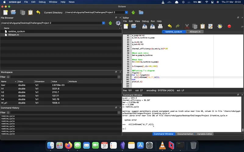
solved by adding ')'
error: scalar cannot be indexed with .
error: called from
rankine_cycle at line 109 column 4
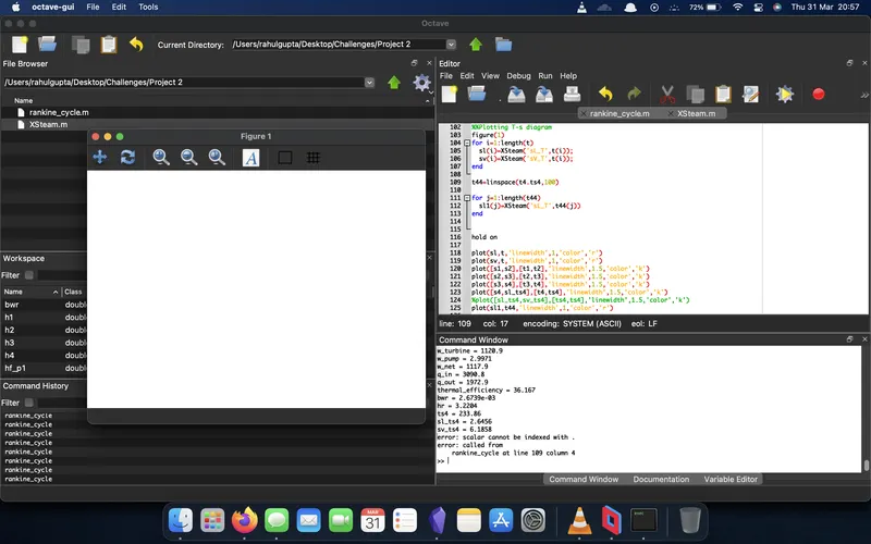
solved by changing '.' to ','
References
Engineering Thermodynamics - P.K. Nag