Week 4.1 - Genetic Algorithm

Genetic Algorithm studies:

clear all
close all
clc

% Creating meshgrid to plot stalgamite function
x = linspace(0,0.6,200);
y = linspace(0,0.6,200);
[xx yy] = meshgrid(x,y);
limit = 150;    % No. of iterations

for i = 1:length(x)
    for j = 1:length(y)
        stal_input(1) = xx(i,j);
        stal_input(2) = yy(i,j);
        z_stal(i,j) = stalagmite(stal_input);
    end
end
% z-values of stalagmite function is now saved in z_stal array

tic

% STUDY 1: No bounds are specified; default population
for i = 1:limit
    
    [input_opt,fopt(i)] = ga(@stalagmite,2);
    xopt(i) = input_opt(1);
    yopt(i) = input_opt(2);
        
end
time_study1 = toc

figure('Name','Study 1: No bounds specified; default population');
subplot(2,1,1)
plot3(xopt,yopt,-fopt,'marker','o')
grid on
hold on
surf(x,y,-z_stal)
shading interp
xlabel('x')
ylabel('y')
zlabel('z')
subplot(2,1,2)
plot(-fopt)

Glo_Max_Nobounds_defpopul = max(-fopt)

% STUDY 2: No bounds are specified; increased population (set to x & y range of the fitness function)

options = optimoptions(@ga,'populationsize',200)
tic

for i = 1:limit
    
    [input_opt,fopt(i)] = ga(@stalagmite,2,[],[],[],[],[],[],[],options);
    xopt(i) = input_opt(1);
    yopt(i) = input_opt(2);
        
end
time_study2 = toc

figure('Name','Study 2: No bounds; increased population');
subplot(2,1,1)
plot3(xopt,yopt,-fopt,'marker','o')
grid on
hold on
surf(x,y,-z_stal)
shading interp
xlabel('x')
ylabel('y')
zlabel('z')
subplot(2,1,2)
plot(-fopt)

Glo_Max_Nobounds_200_popul = max(-fopt)

% STUDY 3: Bounds are specified; default population (set to x & y range of the fitness function)
for i = 1:limit
    
    [input_opt,fopt(i)] = ga(@stalagmite,2,[],[],[],[],[0 0],[0.6 0.6]);
    xopt(i) = input_opt(1);
    yopt(i) = input_opt(2);
        
end
time_study3 = toc

figure('Name','Study 3: Bounds are specified; default population');
subplot(2,1,1)
plot3(xopt,yopt,-fopt,'marker','o')
grid on
hold on
surf(x,y,-z_stal)
shading interp
xlabel('x')
ylabel('y')
zlabel('z')
subplot(2,1,2)
plot(-fopt)

Glo_Max_Bounds_defpopul = max(-fopt)


% STUDY 4: Bounds are specified; 200 population (set to x & y range of the fitness function)

options = optimoptions(@ga,'populationsize',200)

for i = 1:limit
    
    [input_opt,fopt(i)] = ga(@stalagmite,2,[],[],[],[],[0 0],[0.6 0.6],[],options);
    
    xopt(i) = input_opt(1);
    yopt(i) = input_opt(2);
        
end
time_study4 = toc

figure('Name','Study 4: Bounds are specified; 200 population');
subplot(2,1,1)
plot3(xopt,yopt,-fopt,'marker','o')
grid on
hold on
surf(x,y,-z_stal)
shading interp
xlabel('x')
ylabel('y')
zlabel('z')
subplot(2,1,2)
plot(-fopt)

Glo_Max_Bounds_200popul = max(-fopt)
disp("Global Maximum by")
disp("Study1 = "+ Glo_Max_Nobounds_defpopul)
disp("Study2 = "+ Glo_Max_Nobounds_200_popul)
disp("Study3 = "+ Glo_Max_Bounds_defpopul)
disp("Study4 = "+ Glo_Max_Bounds_200popul)

Stalagmite function:

function [F] = stalagmite(input_vector)
x = input_vector(1);
y = input_vector(2);

f1x = (sin(5.1*pi*x + 0.5)).^6;
f1y = (sin(5.1*pi*y + 0.5)).^6;

f2x = exp(-4*log(2)*(((x-0.0667).^2)/(0.64)));
f2y = exp(-4*log(2)*(((y-0.0667).^2)/(0.64)));

[F] = -1*f1x*f2x*f1y*f2y;
end

Concept of Genetic Algorithm:

Genetic algorithms are based on the ideas of natural selection and genetics. Genetic algorithms simulate the process of natural selection they simulate “survival of the fittest”. The population of individuals are maintained within search space. Each individual represents a solution in search space for given problem. Each individual is coded as a finite length vector of components.

1) Selection Operator: The idea is to give preference to the individuals with good fitness scores and allow them to pass their genes to successive generations.
2) Crossover Operator: This represents mating between individuals. Two individuals are selected using selection operator and crossover sites are chosen randomly.
3) Mutation Operator: The key idea is to insert random genes in offspring to maintain the diversity in the population to avoid premature convergence.

1. The whole algorithm can be summarized as:
   1) Randomly initialize populations
   2) Determine fitness of population
   3) Until convergence repeat:
   1. Select parents from population
   2. Crossover and generate new population
   3. Perform mutation on new population
   4. Calculate fitness for new population

ga syntax in Matlab:

x = ga (fun,nvars,A,b,Aeq,beq,lb,ub,nonlcon) subjects the minimization to the constraints defined in nonlcon. The function nonlconaccepts x and returns vectors C and Ceq, representing the nonlinear inequalities and equalities respectively. ga minimizes the fun such thatC(x) ≤ 0 and Ceq(x) = 0.

x is the fitness function; lb & ub are upper and lower bounds.
Fitness limit, population size, crossover function,etc. can be set using options.

Stepwise explaination:

1. Creation of meshgrid of x and y value to plot stalagmite function.
2. Use of for loop to input value of meshgrid to stalagmite function and get an array z-values.
3. Use ga solver to get optimum x & y values and optimum fitness value. ga solver needs fitness function & no. of variables as input.
4. For study 1, no bounds are set and population is not specified & set as default (i.e. 50).
5. Plotting: In the same figure window, two axes are created.
   On first axes, surface plot of stalagmite function & 3d plot of ga output are plotted.
   On second axes, optimum fitness values are plotted with interations on x-axis.
6. For study 2, no bounds are set but population is set to 200.
7. For study 3, bounds are set to 0 to 0.6 on both axes with default population.
8. For study 4, same bounds are set with population increased to 200.
9. Global maximum output of each cases are displayed at the end.

Errors faced:

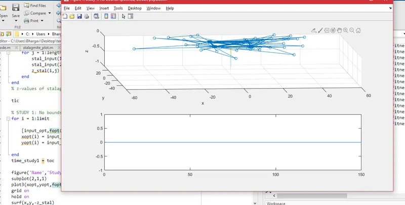
1. Plotting error: Plot of ga fitness values got inverted.
   Fixed it by adding negative sign to fopt.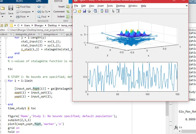
2. Stalagmite z-values were positive, so ga solver plotted scattered values of fopt as the minimum global maximum, in this case, were large amount of floor values of stalagmite function.