Project 2 - Rankine cycle Simulator

clear all
close all
clc

fprintf('RANKINE CYCLE SIMULATOR\n')
fprintf('1-2 Isentropic expansion in the turbine\n')
fprintf('2-3 Constant pressure heat rejection by the condenser\n')
fprintf('3-4 Isentropic compression in the pump\n')
fprintf('4-1 Constant pressure heat addition in boiler\n')

% p: Pressure (bar)             T: Temperature (°C)
% h: Specific enthalpy (kJ/kg)  s: Specific entropy (kJ/kgK)

% Known inputs:
p1 = 30;    % Turbine inlet pressure
T1 = 400;   % Turbine inlet temperature
p2 = 0.05;  % Turbine outlet pressure = Condenser inlet pressure

% STATE 1:
h1 = XSteam('h_pT',p1,T1);
s1 = XSteam('s_pT',p1,T1);

% STATE 2:
s2 = s1;
sf2 = XSteam('sL_p',p2);    % Saturated liquid entropy
sg2 = XSteam('sV_p',p2);    % Saturated vapour entropy
x = (s2-sf2)/(sg2-sf2);     % Dryness fraction
hf2 = XSteam('hL_p',p2);    % Saturated liquid enthalpy
hg2 = XSteam('hV_p',p2);    % Saturated vapour enthalpy
h2 = hf2 + x*(hg2-hf2);
T2 = XSteam('T_ph',p2,h2);

% STATE 3:
p3 = p2;
T3 = T2;
h3 = XSteam('hL_p',p3);
s3 = XSteam('sL_p',p3);

% STATE 4:
p4 = p1;
s4 = s3;
T4 = XSteam('T_ps',p4,s4);

% Calculating Wp,Wt,Wnet,Thermal efficiency,SSC:
v3 = XSteam('v_ps',p3,s3);          % Specific volume
Wp = v3*(p1-p2)*100;                % Pump work
h4 = Wp + h3;
Wt = h1 - h2;                       % Turbine work
Wnet = Wt - Wp;                     % Net work done
T_efficiency = Wnet/(h1-h4);        % Thermal efficiency
SSC = 3600/Wnet;                    % Specific steam consumption

% Defining arrays and values for plotting:
Temp = linspace(1,375,500);         % Temperature array used for plotting

for i= 1:length(Temp)               
    
    sf(i) = XSteam('sL_T',Temp(i));     % Saturated liquid entropy array
    sg(i) = XSteam('sV_T',Temp(i));     % Saturated vapour entropy array
    hf(i) = XSteam('hL_T',Temp(i));     % Saturated liquid enthalpy array
    hg(i) = XSteam('hV_T',Temp(i));     % Saturated vapour enthalpy array
end

s5 = XSteam('sL_p',p1);         % Saturated liquid entropy at p1
s6 = XSteam('sV_p',p1);         % Saturated vapour entropy at p1
T5 = XSteam('T_ps',p1,s5);      % Temperature at s5 & p1
T6 = T5;                        % Saturated vapour temperature for p1

% For the curve between s5 & s1:
T = linspace(T1,T5,500);        % Temperature array used for plotting

for i = 1:length(T)
    s_5to1(i) = XSteam('s_pT',p1,T(i));
end

% Plotting T-s diagram:
plot([sf sg],[Temp Temp],'color',[0 0.5 1],'linewidth',1.5)
hold on
plot([s1 s2 s3 s4 s5],[T1 T2 T3 T4 T5],'color',[1 0.5 0.17],'linewidth',1.5)
plot(s_5to1,T,'color',[1 0.5 0.17],'linewidth',1.5)
text(s1,T1-10,'  1')
text(s2,T2,'  2')
text(s3,T3-10,'  3')
text(s4,T4+30,'4')
text(4,250,'P1')
text(4,48,'P2')
text(3,T2+3,'\leftarrow')
text(5.5,T5+3,'\rightarrow')
legend('Saturated curve','Cycle for input values')
xlabel('Specific Entropy (kJ/kgK)')
ylabel('Temperature (°C)')
ylim([0 450])
title('T-s diagram')

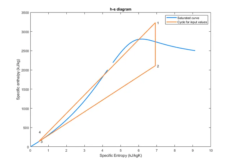
% Plotting h-s diagram:
figure
plot([sf sg],[hf hg],'linewidth',2,'color',[0 0.5 1])
hold on
plot([s1 s2 s3 s4 s1],[h1 h2 h3 h4 h1],'linewidth',2,'color',[1 0.5 0.17])
text(s1,h1,'  1')
text(s2,h2,'  2')
text(s3,h3,'  3')
text(s4,h4+250,'4')
legend('Saturated curve','Cycle for input values')
xlabel('Specific Entropy (kJ/kgK)')
ylabel('Specific enthalpy (kJ/kg)')
title('h-s diagram')

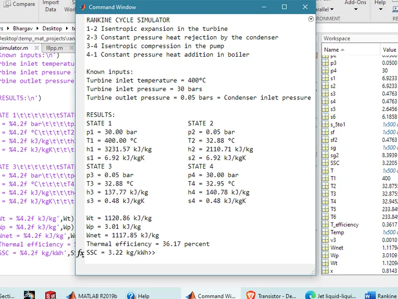
% Printing:
fprintf('\nKnown inputs:\n')
fprintf('Turbine inlet temperature = 400°C\n')
fprintf('Turbine inlet pressure = 30 bars\n')
fprintf('Turbine outlet pressure = 0.05 bars = Condenser inlet pressure\n')

fprintf('\nRESULTS:\n')

fprintf('STATE 1\t\t\t\t\t\tSTATE 2\n')
fprintf('p1 = %4.2f bar\t\t\t\tp2 = %4.2f bar\n',p1,p2)
fprintf('T1 = %4.2f °C\t\t\t\tT2 = %4.2f °C\n',T1,T2)
fprintf('h1 = %4.2f kJ/kg\t\t\th2 = %4.2f kJ/kg\n',h1,h2)
fprintf('s1 = %4.2f kJ/kgK\t\t\ts2 = %4.2f kJ/kgK\n',s1,s2)

fprintf('STATE 3\t\t\t\t\t\tSTATE 4\n')
fprintf('p3 = %4.2f bar\t\t\t\tp4 = %4.2f bar\n',p3,p4)
fprintf('T3 = %4.2f °C\t\t\t\tT4 = %4.2f °C\n',T3,T4)
fprintf('h3 = %4.2f kJ/kg\t\t\th4 = %4.2f kJ/kg\n',h3,h4)
fprintf('s3 = %4.2f kJ/kgK\t\t\ts4 = %4.2f kJ/kgK\n',s3,s4)

fprintf('\nWt = %4.2f kJ/kg',Wt)
fprintf('\nWp = %4.2f kJ/kg',Wp)
fprintf('\nWnet = %4.2f kJ/kg',Wnet)
fprintf('\nThermal efficiency = %4.2f percent',T_efficiency*100)
fprintf('\nSSC = %4.2f kg/kWh',SSC)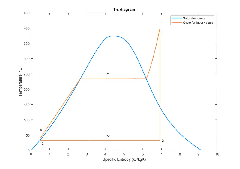

Simple Rankine Cycle:
The simple Rankine cycle is also a reversible cycle.

Principal components of Rankine cycle:
The four basic components of a Rankine cycle are shown in figure. Each component in the cycle is regarded as a control volume, operating at steady state.

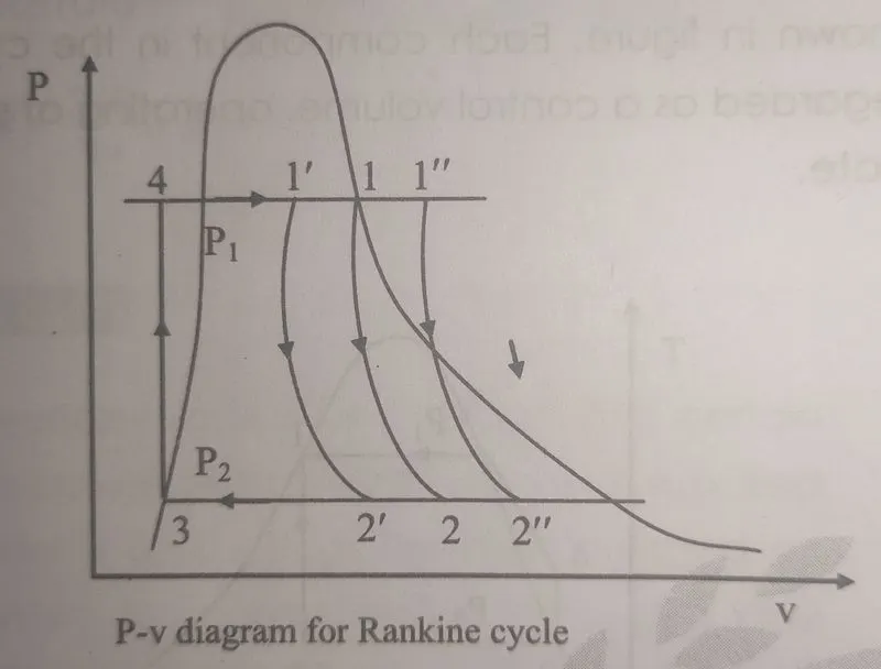
1. Boiler: The heat is supplied to the working fluid (feed water) in the boiler and thus vapour is generated. The vapour leaving the boiler is either saturated at the state 1 or superheated at the state 1", depending upon the amount of heat supplied in the boiler.

2. Turbine: The vapour leaving the boiler enters the turbine, where it expands isentropically to the condenser pressure at the state 2. The work produced by the turbine is rotary (shaft) work and is used to drive an electric generator or machine.

3. Condenser: The condenser is attached at the exit of the turbine. The vapour leaving the turbine is wet vapour and it is condensed completely in the condenser to the state 3, by giving its latent heat to some other cooling fluid like water.

4. Pump: The liquid condensate leaving the condenser at the state 3 is pumped to the operating pressure of the boiler. The pump operation is considered isentropic.

The various processes in simple rankine cycle are:

1-2: Isentropic expansion (Reversible adiabatic expansion of steam in steam turbine)
2-3: Constant pressure heat rejection (constant pressure heat rejection in the condenser to convert condensate into water)
3-4: Isentropic compression (Water from the condenser at low pressure is pumped into the boiler at high pressure. This process is reversible adiabatic
4-1: Constant pressure heat supply (Water is converted into steam at constant pressure Show (the by the addition of heat in the boiler)

The illustration of a steam power plant operating on simple Rankine cycle is shown in P-v, T-s and h-s diagram:

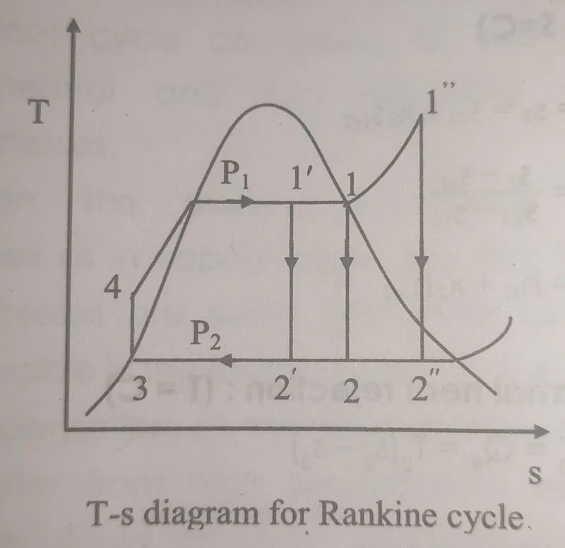
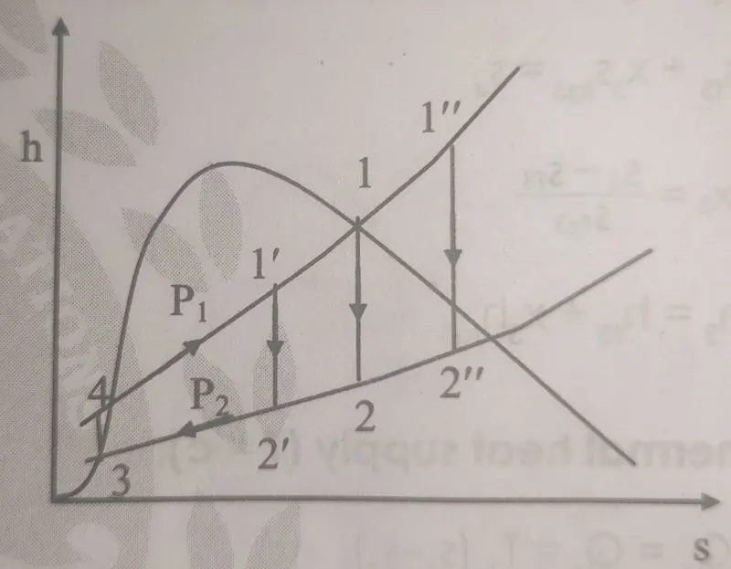
The steam leaving from boiler may be dry and saturated, wet or superheated. The corresponding T-s diagrams are 1-2-3-4-1, 1¹-2’ 3-4-1' or 1"-2"-3-4-1".

Analysis of Rankine cycle:
We assume 1kg of working substance in the cycle and applying steady flow energy equation to each component in the cycle. If changes of kinetic energy and potential energy are neglected then the steady-flow energy equation reduces to
q - w= Δh

1-2: Isentropic expansion
w_T = h₁ - h₂

Taking pump work negative, then
w_p = h₄-h₃
where,
h₃ = h_f = enthalpy of liquid at pressure P₂
h₄ = enthalpy of water at state 4
h₄ =h₃ + W_p
Then the isentropic compression work w_p is obtained as is
W_p = v_f(p₁-p₂)
where,
v is the specific volume of liquid at condenser pressure p₂.
Usually the pump work is negligible as the specific volume of water is very less.

2-3: Constant pressure heat rejection
Q₂₃ = h₃ -h₂
Taking negative sign for heat rejection, then
Q₂₃ = h₂ -h₃

3-4: Isentropic compression
W_p = h₄-h₃

4-1: Constant pressure heat supply
Q₄₁=h₁ -h₄
Since The thermal efficiency of any power cycle is expressed as
η = (Net work done in cycle)/(Heat supplied in the cycle = W_net/Q_in

For Rankine cycle,
W_net = W_T - W_p = (h₁ - h₂) - v_f(p₁ - p₂)
For thermodynamic cycle, the net work is also equal to net heat transfer:
W_net = Q_in - Q_out = (h₁-h₂)-(h₂-h₂)

Step-wise explaination:

1. We use Xsteam.m function file to get the data from it using command, XSteam(fun,In1,In2)
2. Create variables for each state, p: Pressure; T: Temperature; h: Specific enthalpy s: Specific entropy
   followed by 1,2,3 or 4 for its state.
3. First we mention known inputs, p1,T1,p2.
4. Get h1 & s1 values using Xsteam function for state 1.
5. Calculate dryness fraction,x using sf(Saturated liquid entropy) & sg(Saturated vapour entropy) at state 2.
6. Calculate h2 using x, and get T2 from Xsteam.
   Similarly values of h3, s3, T4 are extracted from Xsteam.
7. Calculation of Wt, Wp, Wnet, Thermal efficiency, SSC using mathematical formulae.
8. Creating arrays & points for plotting:
   Temperature array is created using linspace from 1 to 375.
   Using for loop, saturation values of entropy and enthalpy at liquid & vapour states are filled in respective arrays using Xteam.
9. For plotting T-s diagram, saturated liquid entropy at p1, saturated vapour entropy at p1, temperature at s5 & p1, saturated vapour temperature for p1 are taken fom Xsteam.
   Plotting curve form s5 to s1: Temp array is created from T5 to T1. For loop is used to fill entopy values at p1 and temperature, ranging from T5 to T1, using Xsteam.
10. Plotting:
    T-s: Lines are plotted betweem s1 to s5 points & T1 to T5 points, giving it colour, lables, titles, numbering, arrows denoting directin of flow.
    h-s: Lines are plotted between s1 to s4 points & h1 to h4 points, giving it same the same graphical properties.
11. Printing: Using fprintf to show in command window values of thermodynamic properties at 4 different states. And calculated values of Wt, Wp, Wnet, Thermal efficiency, SSC.

Errors faced:

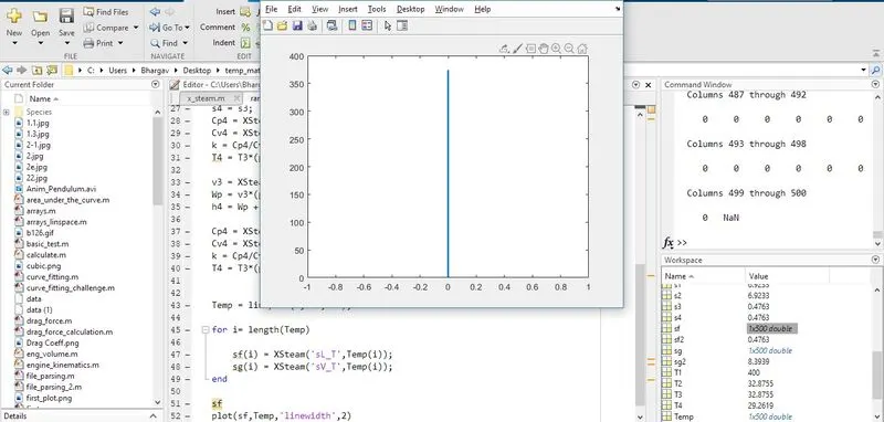
1. Mistake in filling up sf, sg, hf, hg values which created improper graph.
   
2. Typos!!