Week 4.1 - Genetic Algorithm
Objective : To Write a code in MATLAB to optimise the stalagmite function and to find the global maxima of the function.
THEORY :
The genetic algorithm GA is a method for solving both constrained and unconstrained optimisation problems that is based on natural selction,the process that drives biological evolution.
GA repeatedly modifies the population of individual solutions.
At each step, the genetic algorithm selects individuals at random from the current population to be parents and uses them to produce children for the next generation. Over successive generations, the popultation evolves towards an optimal solution.
GA can be applied to solve a variety of optimization problems that are not well suited for standard optimazation algorithms, including problems in which the objective function is discontinuous, non differentiable, stochastic, or highly non linear.
The GA uses 3 main types of rules at each step to create the next gerneration from the current population :
•Selection rule selects the individuals, called parents, that contribute to the population at the next generation.
•crossover rules combine two parents to form children for the next generation.
•Mutation rules apply random changes to individual parents to form children.
PROCEDURE:
1. Initially stalagmite function is defined in a seperate script.
2. A negative sign is used in front of the function to obtain maxima of the function rather minima.
3. A nested for loop is utilized to iterate each of the elements .
4. GA is used to determine the optimal of the function.
5. Plot is generated for different cases.
The three cases considered are :
1. Unbounded inputs
2. Bounded Inputs - restricted with upper and lower bounds
3. Bounded inputs with options - increasing no of iterations by giving population size.
Syntax of ga in MATLAB:
The inbuilt function ga is used to find the global minimum of the function. In order to find the global maxima take the negative of function.
Syntax for ga: [x,fval] = ga(fun,nvars,A,b,Aeq,beq,lb,ub,nonlcon,options)
•x- Minimum value to the function(fun).
•fval- Fitness value.
•ga- Inbuilt function name for calculating genetic algorithm.
•fun- Function handle.
•nvars- Number of variables.
•A,b- Matrix with linear inequalities.
•Aeq,beq- Matrix with linear equalities.
•lb- Lower bound of x.
•ub- upper bound of x.
•Nonlcon- Accept x and gives non linear equalities and inequalities C, Ceq.
•Options- minimize x value with optimization parameters replaced by values in options. Options are created by function optimoptions.
•‘[]’ can be used to fill if any input arguments doesn’t exist.
STALAGMITE FUNCTION :
function [f]=stalagmite(input_vector)
x=input_vector(1);
y=input_vector (2);
f1=(sin(5.1*pi*x+0.5))^6;
f2=(sin(5.1*pi*y+0.5))^6;
f3=exp(-4*log(2)*(x-0.0667)^2/0.64);
f4=exp(-4*log(2)*(y-0.0667)^2/0.64);
f=-(f1*f2*f3*f4);
end
Explaining the code:
•Line 3: Defining the function with function name, input arguments and output variable.
•Line 4-5: Each value of x1 and y1 are stored into x & y for the calculation.
•Line 8-12: Formulas to calculate the stalagmite function.
•Line 14: End command to stop the function.
MAIN CODE:
close all
clc
clear all
%Program to find the global maxima
%Defining the search space
x= linspace(0,0.6,150);
y= linspace(0,0.6,150);
%Creating the 2d array
[x1,y1]=meshgrid(x,y);
%Iteration
num_cases=50;
%Evaluating the stalagmite function
for i=1:length(x1)
for j=1:length(y1)
input_vector(1)=x1(i,j);
input_vector(2)=y1(i,j);
f(i,j)=stalagmite(input_vector);
end
end
%Study 1- Statistical behaviour
tic
for i=1:num_cases
[inputs,fopt(i)]=ga(@stalagmite,2);
xopt(i)=inputs(1);
yopt(i)=inputs(2);
end
study1_time=toc %Timer for evaluating the study 1
figure(1)%New figure window
subplot(2,1,1)%Opening a subplot in same figure
hold on
surf(x1,y1,-f)%Plotting surface
shading interp %Eliminating the grid
plot3(xopt,yopt,-fopt,'marker','o','markersize',5,'markerfacecolor','r')%Plotting the optimum points.
title('Unbounded inputs')
subplot(2,1,2)
plot(-fopt)%Plotting fopt vs iterations
xlabel('Iterations')
ylabel('Function minimum')
%Study 2- Statistical behaviour- with lower and upper bounds
tic
for i=1:num_cases
[inputs,fopt(i)]=ga(@stalagmite,2,[],[],[],[],[0 0],[0.4 0.4]);
xopt(i)=inputs(1);
yopt(i)=inputs(2);
end
study2_time=toc
figure(2)
subplot(2,1,1)
hold on
surf(x1,y1,-f)
shading interp
plot3(xopt,yopt,-fopt,'marker','o','markersize',5,'markerfacecolor','r')
title('Bounded inputs')
subplot(2,1,2)
plot(-fopt)
xlabel('Iterations')
ylabel('Function minimum')
%Study 3 - increasing the ga iterations
tic
options= optimoptions('ga','populationsize',200);
for i=1:num_cases
[inputs,fopt(i)]=ga(@stalagmite,2,[],[],[],[],[0 0],[0.3 0.3],[],[],options);
xopt(i)=inputs(1);
yopt(i)=inputs(2);
end
study3_time=toc
figure(3)
subplot(2,1,1)
hold on
surf(x1,y1,-f)
shading interp
plot3(xopt,yopt,-fopt,'marker','o','markersize',5,'markerfacecolor','r')
title('Bounded inputs with modified population size')
subplot(2,1,2)
plot(-fopt)
xlabel('Iterations')
ylabel('Function minimum')
Explaining the code:
•Line 7-8: Creating search space with 1 dimensional array and storing in x &y.
•Line 10: Creating 2D array using the 1D arrays.
•Line 12: Iteration
•Line 14-15: Starting the for loop for value of x1 & y1. Loop counter is i & j.
•Line 16-17: Calling each value from x1 and y1 as the for loop goes.
•Line 18: Calling the function and giving the inputs collected from line 16-17 to the function. Each function value is collected and an array is formed.
•Line 19-20: End command for both For Loop.
Study 1- Statistical behaviour
•Line 23: Tic and toc command to check the time of study1
•Line 24: For loop for finding the optimum value of function.
•Line 25: Calling the function ga with function handle and number of variable in function.
•Line 26-27: Taking the x optimum & y optimum value from inputs.
•Line 28: For loop ends.
•Line 29: Gives the time of running.
•Line 30: Opens figure window.
•Line 31: subplot command used to open multiple plots in same figure window.
•Line 32: Hold on command used to retain the plots on current axis without deleting the existing plot when new plots are added.
•Line 33: surf command to plot 3D with surface for stalagmite function.
•Line 34: shading interp command to get rid of the grid in surface plot.
•Line 35: plot3 command to plot the optimum values that the ga produce over the 50 cases(iteration).
•Line 36: Title for figure window given.
•Line 37-38: Next subplot created for plotting iteration Vs function minimum.
•Line 39-40: Labelling the x & y axis.
Study 2- Statistical behaviour- with lower and upper bounds.
•Line 43: Timer starts with tic command.
Line 44-48: For loop starts with counter number of cases. Function ga calls the stalagmite function with 2 variables and having a lower and upper bounds to filter the fmin(function minimum) values to the range.
•Line 49: Timer for study2 ends with toc command and displayed in command window.
•Line 50-60: Again the same stalagmite function plot is displayed as above study, but this time the function minimum values are filtered to 3 points.
Study 3 – Increasing the ga iterations.
•Line 63: Timer for study 3.
•Line 64: Function optimoptions is used to give the population size to ga.
•Line 65-69: For loop for finding the foptimum.
•Line 70: Time took to run this study is displayed on command window.
•Line71-81: Stalagmite function plot is done.
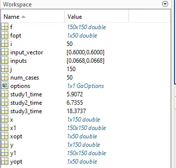
OUTPUT:
RESULT:
Study 1
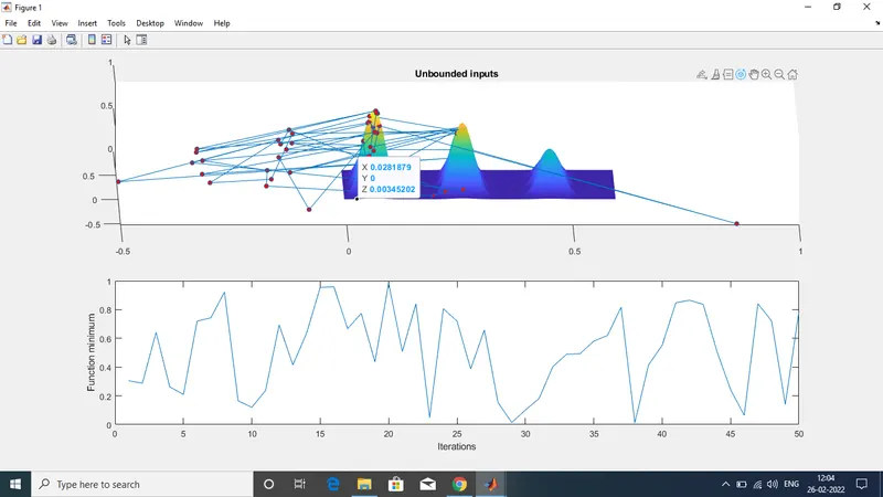
In study 1 getting ga predicts different minimum values for the function. It’s because the ga takes random sampling.
Study 2
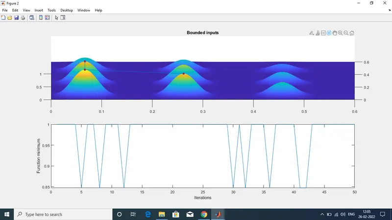
Study 2: In study 1 the variables x & y are going beyond 0.6 and less than 0 to negative. To filter it lower and upper bounds are given. Here we can see that the function minimum is filtered to 3 points. But here when giving the upper and lower bounds we have to give a good guess or know the function properly, so that the bounds are given correctly to get the minimum.
study 3
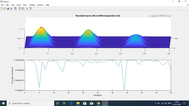
Study 3 is done with bounded inputs and increasing the population size. Increasing the population can find the global minima.
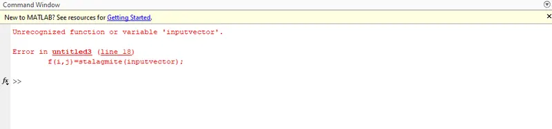
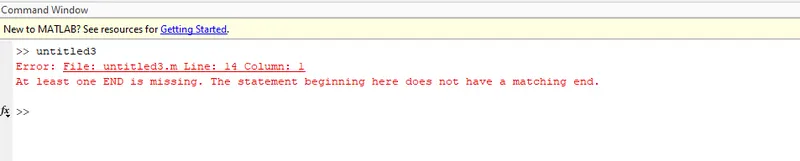
ERROR FACED: