Week 4.1 - Genetic Algorithm

- x = ga(fun,nvars,A,b) finds a local minimum x to fun, subject to the linear inequalities A*x ≤ b. ga evaluates the matrix product A*x as if x is transposed (A*x').

- x = ga(fun,nvars,A,b,Aeq,beq) finds a local minimum x to fun, subject to the linear equalities Aeq*x = beq and A*x ≤ b. (Set A=[] and b=[] if no linear inequalities exist.) ga evaluates the matrix product Aeq*x as if x is transposed (Aeq*x').

- x = ga(fun,nvars,A,b,Aeq,beq,lb,ub) defines a set of lower and upper bounds on the design variables, x, so that a solution is found in the range lb ≤ x ≤ ub. (Set Aeq=[] and beq=[] if no linear equalities exist.)

- x = ga(fun,nvars,A,b,Aeq,beq,lb,ub,nonlcon) subjects the minimization to the constraints defined in nonlcon. The function nonlcon accepts x and returns vectors C and Ceq, representing the nonlinear inequalities and equalities respectively. ga minimizes the fun such that C(x) ≤ 0 and Ceq(x) = 0. (Set lb=[] and ub=[] if no bounds exist.)

- x = ga(fun,nvars,A,b,Aeq,beq,lb,ub,nonlcon,options) minimizes with the default optimization parameters replaced by values in options. (Set nonlcon=[] if no nonlinear constraints exist.) Create options using optimoptions.

- x = ga(fun,nvars,A,b,Aeq,beq,lb,ub,nonlcon,intcon) or x = ga(fun,nvars,A,b,Aeq,beq,lb,ub,nonlcon,intcon,options) requires that the variables listed in intcon take integer values.

close all
clear all
clc

%Search area inputs
x= linspace(0,0.6,150);
y= linspace(0,0.6,150);
numspace= 50;

%creating a 2 dimensional array
[xx yy] = meshgrid(x,y);

%evaluating the stalagmite function

for i=1:length(x)
   for j=1:length(y)
    input_vector(1)= xx(i,j);
     input_vector(2)= yy(i,j);
     f(i,j)= stalagmite(input_vector);
end
end

%study no. 1 : statistical behavior
tic
for i= 1:numspace
    [result,fopt(i)]= ga(@stalagmite,2)
    xopt(i)= result(1)
    yopt(i)= result(2)
end
study_time1= toc
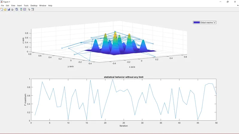
figure(1)
subplot(2,1,1)
surfc(x,y,-f)
shading interp
hold on
plot3(xopt,yopt,-fopt,'marker','o','markersize',5)
xlabel('x axis')
ylabel('y axis')
zlabel('z axis')
legend('Global maxima "o"')
subplot(2,1,2)
plot(-fopt)
xlabel('Iteration')
ylabel('F maximum')
title('statistical behavior without any limit')



%study no. 2 : statistical behavior with upper and lower limit

tic
for i=1:numspace
    [result, fopt(i)]= ga(@stalagmite,2,[],[],[],[],[0 0],[0.6 0.6])
    xopt(i)= result(1)
    yopt(i)= result(2)
end
study_time2= toc
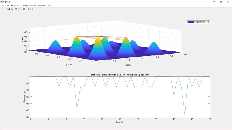
figure(2)
subplot(2,1,1)
surfc(x,y,-f)
shading interp
hold on
plot3(xopt,yopt,-fopt,'marker','o','markersize',5)
xlabel('x axis')
ylabel('y axis')
zlabel('z axis')
legend('Global maxima "o"')
subplot(2,1,2)
plot(-fopt)
xlabel('Iteration')
ylabel('F maximum')
title('statistical behavior with  and lower limit')

%study no. 3 : increasing "ga" iterations from 50 to 300

tic
options= optimoptions('ga')
options= optimoptions(options,'populationsize',300)
for i=1:numspace
    [result,fopt(i)]= ga(@stalagmite,2,[],[],[],[],[0 0],[0.6 0.6],[],[],options)
    xopt(i)= result(1)
    yopt(i)= result(2)
end
study_time3= toc
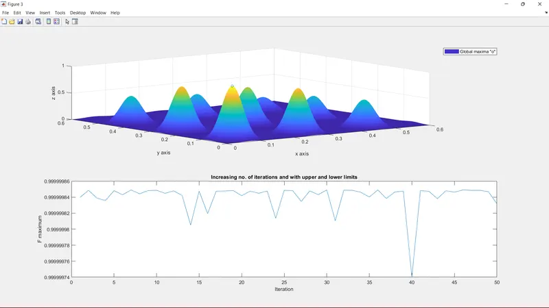
figure(3)
subplot(2,1,1)
surf(x,y,-f)
shading interp
hold on
plot3(xopt,yopt,-fopt,'marker','o','markersize',5)
xlabel('x axis')
ylabel('y axis')
zlabel('z axis')
legend('Global maxima "o"')
subplot(2,1,2)
plot(-fopt)
xlabel('Iteration')
ylabel('F maximum')
title('Increasing no. of iterations and with upper and lower limits')

3) Output for each study are shown below respectively.

Study no. 1

Study no. 2

Study no. 3

4) Stepwise explanation of code.

Starting with basic commands close all, clear all, clc

Entering search area inputs in "x" and "y" variable, "numspace" gives number of iterations to perform.

Creating 2D array out of "x" and "y" values using "meshgrid()" command and assigning values to "xx", "yy". These "xx", "yy" values then assigned to input_vector(1) and input_vector(2).

calling a function "stalagmite(input_vector)" for which different code has been written and its value been saved in variable "f(i,j)".

In study no. 1

"tic" start to count time require to solve genetic algorithm.

In for loop "i" for each value of numspace i.e. itteration number genetic algorithm command is itterated having function handle "stalagmite" with two variables "x and y", each itteration value are saved in "result" and "fopt()".

"xopt" and "yopt" takes "x" and "y" values from result, "fopt" has value global maxima value.

"study_time1= toc" counts total time taken and displays it.

plotting all values simultaniously using respective commands, here "-fopt" is used to actually get global maxima.

For study number 2.

The only difference in "ga" is syntax in which upper and lower boundries are set to get some accurate global maxima values. Rest all remains same.

For study number 3.

"optimoptions()" command is used to optimise "ga" by increasing population size to 300 and adding "option" in "ga" syntax.

so we get only one value of global maxima. Again rest all remains same.

5) code for "stalagmite" function

function [F]= stalagmite(input_vector)

 x= input_vector(1);
 y= input_vector(2);
f1x= (sin((5.1*x*pi) + 0.5)).^6;
f2x= exp((-4*log(2))*((x-0.0667).^2/0.64));
f1y= (sin((5.1*y*pi) + 0.5)).^6;
f2y= exp((-4*log(2))*((y-0.0667).^2/0.64));

F= -(f1x* f2x* f1y* f2y);
end

explanation for above code

In variable "F" "stalagmite" is function name "input_vector" are input parameters i.e. "x" and "y" for which function will be solved.

f1x, f2x, f1y, f2y are written with their respective equations.

"F" has a product of above equation with "-" sign so that actual global maxima value is obtained.