Project 2 - Rankine cycle Simulator

Matlab code to simulate Rankin cycle.

1) Rankin cycle: It is a modification of Carnot cycle. Its a ideal cycle on which a steam engine works. It consist of following process.

1-2: Adiabatic expansion- In turbine dry steam is expanded adiabatically to pressure p2.

2-3: Constant pressure heat rejection- In condenser, heat is rejected at constant pressure p2. Only latent heat is removed. Steam is condensed to saturated water.

3-3': Adiabatic compression- Water is fed to the boiler by a pump. During pumping pressure of water is increased from p2 to p1.

3-4: Constant pressure heat addition- In economiser, heat is added to water . Its temperature is increased to saturetion temperature at constant pressure p1.

4-1: Constant pressure heat addition- In boiler heat is added to saturated water. It evaporates into dry steam at constant pressure p1. Steam flows to turbine and cycle is repeated.

2) Code to read XSteam data and simulate the cycle.

clear all
close all
clc

%to display cycle name and its stages 
fprintf('RANKIN CYCLE SIMULATOR \n\n')
fprintf('1-2 is Isentropic expansion in the turbine \n')
fprintf('2-3 is constant pressure heat removal in the condenser \n')
fprintf('3-4 is Isentropic compression in the pump \n')
fprintf('4-1 is constant pressure heat addition in the boiler  \n\n')


%for taking an input
P1 = input('Enter the pressure at turbine inlet, P1(in bar) = ');
T1 = input('Enter the temperature at turbine inlet, T1(in degree C) = ');
P2 = input('Enter the pressure at condenser inlet, p2(in bar) =  ');


%reading input data from XSteam.m file
% state 1(Enthalpy(h1) and Entropy(s1))
h1 = XSteam('h_pT', P1, T1);
s1 = XSteam('s_pT', P1, T1);

%state 2  
s2 = s1;
sf2 = XSteam('sL_p',P2);
sg2 = XSteam('sV_p',P2);
x2 = (s2-sf2)/(sg2-sf2);
hf2 = XSteam('hL_p',P2);
hg2 = XSteam('hV_p',P2);
h2 = hf2 + (x2*(hg2-hf2));

%state 3
P3 = P2;
s3 = XSteam('sL_p',P3);
h3 = XSteam('hL_p',P3);

%state 4
s4 = s3;
P4 = P1;

%work done by turbine
Wt = h1 - h2;

%work done to run pump
V3 = XSteam('vL_p',P3);
Wp = V3*(P4 - P3)*100;
h4 = h3 + Wp;

%net work done
Wnet = Wt - Wp;

%heat taken into the system
Qin = h1 - h4;

%heat taken out of the system 
Qout = h2 - h3;

%thermal efficiency
Tef = (Wnet/Qin)*100;

%Specific Steam Consumption(SSC)
SSC = (3600/Wnet);

%calculating temperatures at the state points
T3 = XSteam('Tsat_p',P3);
T2 = T3;
Cp4 = XSteam('Cp_ps',P4,s4);
Cv4 = XSteam('Cv_ps',P4,s4);
k = Cp4/Cv4;
T4 = T3/((P3/P4)^((k-1)/k));

%calculating temperture, enthalpy and entropy
T6 = XSteam('Tsat_p',P1);
if (T6==0)
    printf('The cycle cannot have %f as inlet temperature!!!')
end
s5 = XSteam('sL_p',P1);
s6 = XSteam('sV_p',P1);
h5 = XSteam('hl_p',P1);
h6 = XSteam('hV_p',P1);
T5 = T6;

%plotting the saturation curve
T = linspace(1,400,1000);
for i=1:length(T)
    sf(i) = XSteam('sL_T',T(i));
    sg(i) = XSteam('sV_T',T(i));
    hf(i) = XSteam('hL_T',T(i));
    hg(i) = XSteam('hV_T',T(i));
end

%plotting T-s diagram
figure(1)
hold on
plot(sf,T,'r','linewidth',2)
plot(sg,T,'r','linewidth',2)
plot([s1 s2],[T1 T2],'k','linewidth',2)
plot([s2 s3],[T2 T3],'k','linewidth',2)
plot([s3 s4],[T3 T4],'k','linewidth',2)
plot([s4 s5],[T4 T5],'k','linewidth',2)
plot([s5 s6],[T5 T6],'k','linewidth',2)
sc1 = linspace(s6,s1,2000);
for l = 1:length(sc1)
    Tc1(l) = XSteam('T_ps',P1,sc1(1));
end
plot(sc1,Tc1,'k','linewidth',2)
text(s1+0.1,T1,'1')
text(s2+0.1,T2,'2')
text(s3,T3-20,'3')
text(s4,T4+20,'4')
title('Temperature vs Entropy')
xlabel('Entropy(Kj/KgK)')
ylabel('Temperature (degree C)')
legend('Saturation curve')

%plotting h-s diagram
figure(2)
hold on
plot(sf,hf,'r','linewidth',2)
plot(sg,hg,'r','linewidth',2)
plot([s1 s2],[h1 h2],'k','linewidth',2)
plot([s2 s3],[h2 h3],'k','linewidth',2)
plot([s3 s4],[h3 h4],'k','linewidth',2)
hc = linspace(h4,h5,100);
for k =1:length(hc)
    sch(k) = XSteam('s_ph',P1,hc(k));
end
plot(sch,hc,'k','linewidth',2)
plot([s5 s6],[h5 h6],'k','linewidth',2)
for m =1:length(sc1)
    hc1(m) = XSteam('h_ps',P1,sc1(m));
end
plot(sc1,hc1,'k','linewidth',2)
text(s1+0.1,h1,'1')
text(s2+0.1,h2,'2')
text(s3,h3-100,'3')
text(s4,h4+200,'4')
title('Enthalpy vs Entropy')
xlabel('Entropy (Kj/KgK)')
ylabel('Enthalpy (Kj/Kg)')
legend('Saturation curve')

%to display results
fprintf('\n RESULTS \n\n')

%at stage 1
fprintf('At state point 1: \n')
fprintf('P1 is:%7.3f bar \n',P1)
fprintf('T1 is:%8.3f degree C \n',T1)
fprintf('h1 is:%9.3f Kj/Kg \n',h1)
fprintf('s1 is:%6.3f Kj/KgK \n\n',s1)

%at stage 2
fprintf('At state point 2: \n')
fprintf('P2 is:%6.3f bar \n',P2)
fprintf('T2 is:%7.3f degree C \n',T2)
fprintf('h2 is:%9.3f Kj/Kg \n',h2)
fprintf('s2 is:%6.3f Kj/KgK \n',s2)
fprintf('x2 is:%6.3f \n\n',x2)

%at stage 3
fprintf('At state point 3: \n')
fprintf('P3 is:%6.3f bar \n',P3)
fprintf('T3 is:%7.3f degree C \n',T3)
fprintf('h3 is:%8.3f Kj/Kg \n',h3)
fprintf('s3 is:%6.3f Kj/KgK \n\n',s3)

%at stage 4
fprintf('At state point 4: \n')
fprintf('P4 is:%7.3f bar \n',P4)
fprintf('T4 is:%7.3f degree C \n',T4)
fprintf('h4 is:%8.3f Kj/Kg \n',h4)
fprintf('s4 is:%6.3f Kj/KgK \n\n',s4)

%turbine work
fprintf('Wt is: %7.3f Kj/Kg \n',Wt)
fprintf('Wp is: %5.3f Kj/Kg \n',Wp)
fprintf('Wnet is: %7.3f Kj/Kg \n',Wnet)
fprintf('Efficiency is: %6.3f percent \n',Tef)
fprintf('SSC is: %5.3f Kj/Kwh \n',SSC)

3) Step wise explanation of code.

- Starting with basic comments clear all, close all, clc then using "fprintf()" to print code title and all 4 process at different stages.

- To take inputs from user P1, T1, P2 "input()" command is used.

- Reading enthalpy and entropy from XSteam data for state 1 and saving it in variables h1, s1 respectively for input pressure and temperature given by user.

- At state 2 s2 = s1 as per cycle further reading data for remaining parameters form XSteam file, then finding h2 by using respective formula.

- At state 3 p3 = p2 and reading other parameters form XSteam file.

- At state 4 s4 = s3, p4 = p1 as per cycle.

- Further Wt, Wp, h4, Wnet, Qin, Qout, Tef, SSC are calculated using respective formulas.

- Next finding temperatures, enthalpy and entropy at all state points either from XSteam file or by using formulas.

- Then plotting saturation curve and T-s diagram for 1000 temperature values between 1 to 400 degree C, also indicating state point by using "text()" command.

- Plotting h-s diagram similarly as T-s.

- At the end printing all the parameters in command window using "fprintf()".

4) Output

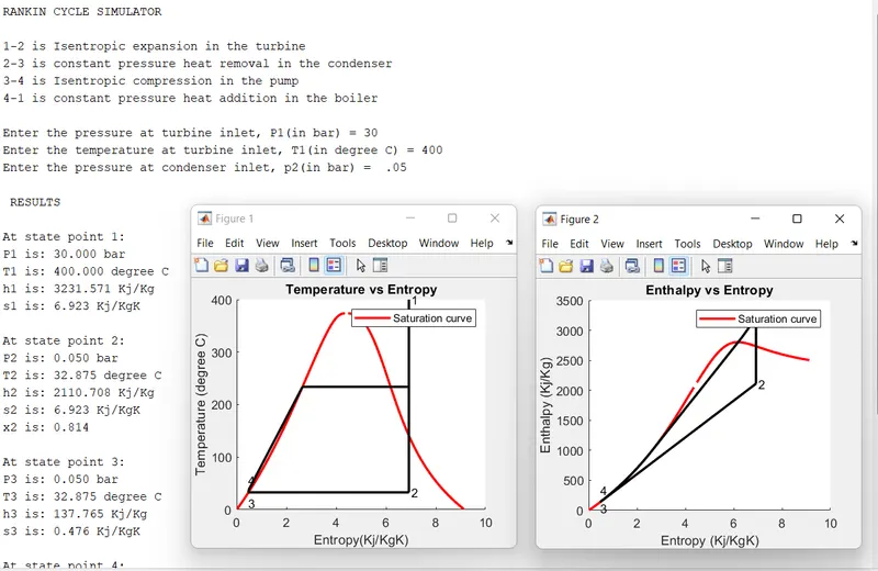
5) Errors.

Errors occured were typo errors that were corrected by reading warnings in command window. Tried to bring same output screen as shown by using "\n" and "%f".