Challenge

Week 4.1 - Genetic Algorithm

It is method for solving both constrained and unconstrained optimization problems based on a natural selection process that mimics biological evolution.
The algorithm repeatedly modifies a population of individual solutions.
At each step, the genetic algorithm randomly selects individuals from the current population and uses them as parents to produce the children for the next generation.
Over successive generations, the population "evolves" toward an optimal solution.
Genetic algorithm solver for mixed-integer or continuous-variable optimization, constrained or unconstrained.
Genetic algorithm solves smooth or nonsmooth optimization problems with any types of constraints, including integer constraints.
It is a stochastic, population-based algorithm that searches randomly by mutation and crossover among population members.
to under stand GA in HINDI.

How the Genetic Algorithm Works ?

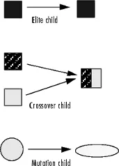
SELECTION = Eliteare the individuals in the current generation with the best fitness values. These individuals automatically survive to the next generation. it means select the individuals. called parant that contribute to the population at the next genration.
CORSSOVER = Crossover are created by combining the vectors of a pair of parents. it means that combine two parants from childrent to next genration.
MUTATION = Mutation children are created by introducing random changes, or mutations, to a single parent. it means that apply random changes to individual parents to from children.

Syntax used in our program

to get more infomation about GA SYNTAX

Using three syntax here for solving my program are as following,

STUDY-1: UNBOUNDED INPUTS : f(i,j) = stalagmite(INPUT_VECTOR)

x = ga(fun,nvars)

[INPUT, fopt(i)] = ga(@stalagmite,2);

x = [INPUT, fopt(i)] = to the objective function,

ga = Find minimum of function using genetic algorithm,

fun. nvars = is the dimension (number of design variables) of fun = stalagmite.

nvars = nvars — Number of variables positive integer, 2 of the function, here it is X and Y for creating 2-d meshing,

this syntax helps to finds a local unconstrained minimum.

STUDY -2 : STATISTICAL BEHAVIOR WITH BOUNDED INPUTS

x = ga(fun,nvars,A,b,Aeq,beq)

[INPUT, fopt(i)] = ga(@stalagmite,2,[],[],[],[],[0;0],[1;1]);

A,B & Aeq,Beq = linear equality constraint.

A = []; linear inequality constraints, real matrix,
b = []; linear inequality constraints, real vector,
Aeq = []; linear equality constraints, real matrix,
beq = []; linear equality constraints, real vector,
lb = []; Lower bounds,[] (default) | real vector or array
ub = [];Upper bounds,[] (default) | real vector or array
nonlcon = []; Nonlinear constraints function handle | function name

this syntax helps to finds a local minimum x to fun,

subject to the linear equalities Aeq*x = beq and A*x ≤ b. (Set A=[] and b=[] if no linear inequalities exist.)

ga evaluates the matrix product Aeq*x as if x is transposed (Aeq*x').

STUDY-3: STATISTICAL BEHAVIOR WITH INCREASING GA ITERATIONS

x = ga(fun,nvars,A,b,Aeq,beq,lb,ub,nonlcon,intcon,options)

[INPUT, fopt(i)] = ga(@stalagmite,2,[],[],[],[],[0;0],[1;1],[],[],options);

@ = defines what function to minimise,

lb = lower bound,

ub = upper bound,

nonlcon = non-linear constraints

intcon = vector of positive integers

option = optimization options output of optimoptions | structure

this syntax helps to minimizes with the default optimization parameters replaced by values in options. (Set nonlcon=[] if no nonlinear constraints exist.)

Create options using optimoptions.

THE BELOW FUNCTION ID BASED ON FOLLOWING FORMULA FOR STALAGMITE

`f(x,y) = f1,xf2,xf1,yf2,y`

`f1.x = [sin(5.1pix + 0.5)]^6` `f1.y = [sin(5.1piy + 0.5)]^6`

`f2,x = exp[-4ln(2)(x-0.0667)^2/0.64]`

`f2,y = exp[-4ln(2)(y-0.0667)^2/0.64]`

STALAGMITE FUNCTION =

%STALAGMITE FUNCTION

function  [y] = stalagmite(INPUT_VECTOR)
    
x = INPUT_VECTOR(1);
y = INPUT_VECTOR(2);

f1 = (sin(5.1*pi*x+0.5)).^6;

f2 = (sin(5.1*pi*y+0.5)).^6;

f3 = exp((-4*log(2)*((x-0.0667)^2))/(0.64));

f4 = exp((-4*log(2)*((y-0.0667)^2))/(0.64));

[y] = -(f1*f2*f3*f4);
end

EXPLNATION :

for performting whole program need function and our function is 'STALAGMITE'.
STALAGMITE saved as seprate program. stalagmite function takes in the data given inside parantheses and calculate.
N = 50 it means that 50cases are assign to run through the stalagmite function & genetic algorithm. it is done for 50 iterations as mentioned to run ga 50 times.
linspace = it hepls to genrate row vector for x and y vector for (0,0.6,150) It Generate linearly spaced vector
meshgrid = it was taking vale from our 2D vector wich was created by using linspace to creat 3d vector (2-D and 3-D grids).The grid represented by the coordinates X and Y has length(y) rows and length(x) columns.
ga = Find minimum of function using genetic algorithm
forloop = for loop to repeat specified number of times
tic toc = tic works with the toc function to measure elapsed time. The tic function records the current time, and the toc function uses the recorded value to calculate the elapsed time.
surf = Contour plot under surface plot
subplot = Create axes in tiled positions
plot3 = 3-D point or line plot. plots coordinates in 3-D space.

In our programd plot3(X,Y,Z) plots coordinates in 3-D space. it is defined as = xopt,yopt,-fopt.

by default in MATLAB, ga calculates the global minima. IN order to make it show the global maxima we add a -ve sign to ,f, and ,fopt' everywhere.

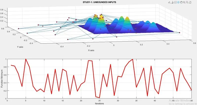
STUDY-1: UNBOUNDED INPUTS

In study 1 syntax was which is helps to finds a local unconstrained minimum.

Study 1 is done for statistical behaviour of the stalagmite function and its values are random and changes and not much optmized.

%STUDY1: UNBOUNDED INPUTS
clear all
close all
clc

%Defining the search space
x = linspace(0,0.6,150);
y = linspace(0,0.6,150);
N = 50 %to run ga 50 times

%Creating 2-D Mesh
[X Y] = meshgrid(x,y);

%Evaluating the stalagamite fuction
for i=1:length(X)
     for j=1:length(Y)
         INPUT_VECTOR(1) = X(i,j);
         INPUT_VECTOR(2) = Y(i,j);
         %Function defination
         f(i,j) = stalagmite(INPUT_VECTOR);
     end
end

tic

for i = 1:N
         [INPUT, fopt(i)] = ga(@stalagmite,2);
         xopt(i) = INPUT(1);
         yopt(i) = INPUT(2);
end

Study1_time = toc

%Plotting the graph
figure(1)
subplot(2,1,1)
hold on
surfc(X,Y,-f)
shading interp;
xlabel('X axis');
ylabel('Y axis');
grid on

title('STUDY-1: UNBOUNDED INPUTS')
plot3(xopt,yopt,-fopt,'marker','o','MarkerSize',5,'MarkerFaceColor','r');
subplot(2,1,2)
plot(-fopt,'LineWidth',3,'Color','r')
xlabel('Iterations')
ylabel('Function Minimum')
grid on

STUDY-1 OUTPUT

STUDY -2 : STATISTICAL BEHAVIOR WITH BOUNDED INPUTS

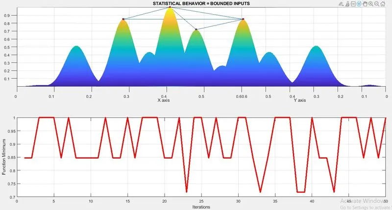
In Study 2 the syntax was used which helps to finds a local minimum.

in this case whole program is similar to study 1 only change in syntax

Study 2 is done for further optimization of the stalagmite function.

%STUDY2: STATISTICAL BEHAVIOR UPPER AND LOWER BOUNDS
clear all
close all
clc

%Defining the search space
x = linspace(0,0.6,150);
y = linspace(0,0.6,150);
N = 50

%Creating 2-D Mesh
[X Y] = meshgrid(x,y);

%Evaluating the stalagamite fuction
for i=1:length(X)
     for j=1:length(Y)
         INPUT_VECTOR(1) = X(i,j);
         INPUT_VECTOR(2) = Y(i,j);

         %Function defination
         f(i,j) = stalagmite(INPUT_VECTOR);
     end
end

tic

for i = 1:N
         [INPUT, fopt(i)] = ga(@stalagmite,2,[],[],[],[],[0;0],[1;1]);
         xopt(i) = INPUT(1);
         yopt(i) = INPUT(2);
end

Study2_time = toc

%Plotting the graph
figure(3)
subplot(2,1,1)
hold on
surfc(X,Y,-f)
shading interp;
xlabel('X axis');
ylabel('Y axis');
grid on
title('STATISTICAL BEHAVIOR = BOUNDED INPUTS')

plot3(xopt,yopt,-fopt,'marker','o','MarkerSize',5,'MarkerFaceColor','r');
subplot(2,1,2)
plot(-fopt,'LineWidth',3,'Color','r')
xlabel('Iterations')
ylabel('Function Minimum')
grid on

STUDY-2 OUTPUT

STUDY-3: STATISTICAL BEHAVIOR WITH INCREASING GA ITERATIONS

study 2 sucessfully optimized the function but it can still be further optumized, hence we did further one more study where we increase the ga population by modifying the syntax for GA and set it to 150 from default 50.

Initially, the time required to run the program is long. we can reduce this time by reducing the limits . Decreasing the population size will get more accurate results.

by using populationsize it helps to represent global maxima was showing in output figure.

%STUDY-3: STATISTICAL BEHAVIOR WITH INCREASING GA ITERATIONS
clear all
close all
clc

%Defining the search space
x = linspace(0,0.6,150);
y = linspace(0,0.6,150);
N = 50

%Creating 2-D Mesh
[X Y] = meshgrid(x,y); 

options = optimoptions('ga')
options = optimoptions(options,'PopulationSize',100);

tic

%Evaluating the stalagamite fuction
for i=1:length(X)
     for j=1:length(Y)
         INPUT_VECTOR(1) = X(i,j); 
         INPUT_VECTOR(2) = Y(i,j);
         %Function defination
         f(i,j) = stalagmite(INPUT_VECTOR);
     end
end

for i = 1:N
         [INPUT, fopt(i)] = ga(@stalagmite,2,[],[],[],[],[0;0],[1;1],[],[],options);
         xopt(i) = INPUT(1);
         yopt(i) = INPUT(2);
end

Study3_time = toc

%Plotting the graph
figure(3)
subplot(2,1,1)
hold on

surfc(X,Y,-f)
shading interp;
xlabel('X axis');
ylabel('Y axis');
grid on
plot3(xopt,yopt,-fopt,'marker','o','MarkerSize',5,'MarkerFaceColor','r');
title('BOUNDED INPUTS WITH MODIFIED POPULATION SIZE')
subplot(2,1,2)
plot(-fopt)
xlabel('Iterations')
ylabel('Function Maximum')
grid on

STUDY-3 OUTPUT

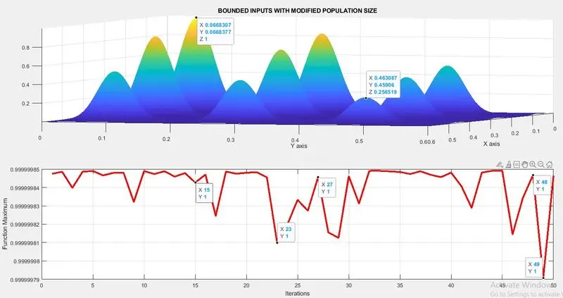
CONCLUSION : the time required to run program is long. we can reduce this time by reducing the limits. Decreasing the population size will get more accurate results.

References :

what is ga in matlab? =

https://in.mathworks.com/discovery/genetic-algorithm.html

https://in.mathworks.com/help/gads/genetic-algorithm.html

Genetic algorithm Terminology ?

https://in.mathworks.com/help/gads/some-genetic-algorithm-terminology.html

How Genetic algorithm works ?

https://in.mathworks.com/help/gads/how-the-genetic-algorithm-works.html