Project 2 - Rankine cycle Simulator
What is Rankine cycle ?
The Rankine cycle is an idealized thermodynamic cycle describing the process by which certain heat engines, such as steam turbines or reciprocating steam engines, allow mechanical work to be extracted from a fluid as it moves between a heat source and heat sink.
Rankine cycle explain ?
Heat energy is supplied to the system via a boiler where the working fluid (typically water) is converted to a high pressure gaseous state (steam) in order to turn a turbine. After passing over the turbine the fluid is allowed to condense back into a liquid state as waste heat energy is rejected before being returned to boiler, completing the cycle. Friction losses throughout the system are often neglected for the purpose of simplifying calculations as such losses are usually much less significant than thermodynamic losses, especially in larger systems.
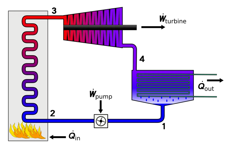
Process and Working :
Process 1-2 is constant pressure heat addition in boiler.
Process 2-3 Isentropic Expansion in the Turbine.
Process 3-4 constant pressure heat rejection in the condenser.
Process 4-1 Isentropic Compression in the pump (Pumping Process).
Rankine cycle Thermal efficiency `ηR` is
`ηtherm`= (Wnet/Qin)*100
above equation can be simplified as following.
Wnet = Wt - Wp
`Wt`= Work done by turbine.
`Wp` = Work done by run pump.
Qin = Heat flow rate to into the system (energy per unit time).
Back Work Ratio : (Wp/Wt).
Specific steam consumtion (S.S.C) : mass flow rate/Wnet; mfw=3600.
FINAL PROGRAM FOR RANKINE CYCLE SIMULATOR
%Rankine cycle simulator
clear all
close all
clc


disp(' RANKINE CYCLE ')
disp('1-2 is Isentropic Expansion in the Turbine');
disp('2-3 is Constant Pressure Heat Rejection by the Condenser');
disp('3-4 is Isentropic Compression in the Pump (Pumping Process)');
disp('4-1 is Constant Pressure Heat Addition in Boiler');

%Obtaining the input data
p1 = input('nValue of Pressure at Turbine Inlet, (in bar) =');                     % p1 = 44;
t1 = input('nValue of Temprature at Turbine Inlet, (in Degree Celcius) =');        % t1 = 538;
p2 = input('nValue of Pressure at Condenser Inlet, (in bar) =');                   % p2 = 5.83;

% variables for stage1
h1 = XSteam('h_pT',p1,t1);                        %Extracting Enthalpy at state pt 1
s1 = XSteam('s_ph',p1,h1);                        %Extracting Enthalpy at state pt 1

fprintf('Results  \n')
fprintf('At state point 1  \n')
fprintf('P1 is:%f bar  \n',p1)
fprintf('T1 is:%f deg celcius  \n',t1)
fprintf('H1 is:%f KJ/Kg \n',h1)
fprintf('S1 is:%f KJ/Kgk \n',s1)

% variables for stage2
s2 = s1;                                          %Isentropic Expansion
t2 = XSteam('T_ps',p2,6.1858);
sf = XSteam('sL_p',p2);                           % Saturated Liquid Entropy
sg = XSteam('sV_p',p2);                           % Saturated Vapour Entropy
hf = XSteam('hL_p',p2);
hg = XSteam('hV_p',p2);
x2 = ((s2 - sf)/(sg - sf));                       %Dryness fraction at state 2
h2 = hf + (x2*(hg - hf));
v2 = XSteam('v_ph',p2,h2);

fprintf('At state point 2 \n')
fprintf('P2 is:%f bar \n',p2)
fprintf('T2 is:%f deg celcius \n',t2)
fprintf('X2 is:%f KJ/Kgk \n',x2)
fprintf('h2 is:%f KJ/Kg \n',h2)
fprintf('S2 is:%f KJ/Kgk \n',s2)


% variables for stage3
t3 = t2;                                          % No subcooling assumeed
p3 = p2;                                          % Constant pressure heat rejection in condenser
s3 = XSteam('sL_p',p3);
h3 = XSteam('hL_p',p3);
v3 = XSteam('v_ph',p3,h3);
fprintf('At state point 3 \n')
fprintf('P3 is:%f bar \n',p3)
fprintf('T3 is:%f deg celcius \n',t3)
fprintf('H3 is:%f KJ/Kg \n',h3)
fprintf('S3 is:%f KJ/Kgk \n',s3)

% variables for stage4
s4 = s3;
v4 = v3;
p4 = p1;
h4 = XSteam('h_ps',p4,s4);
t4 = XSteam('T_hs',h4,s4);
fprintf('At state point 4 \n')
fprintf('P4 is:%f bar \n',p4)
fprintf('T4 is:%f deg celcius \n',t4)
fprintf('H4 is:%f KJ/Kg \n',h4)
fprintf('S4 is:%f KJ/Kgk \n',s4)

% variables for stage5
p5 = p4;
t5 = XSteam('Tsat_p',p5);
h5 = XSteam('hL_T',t5);
s5 = XSteam('sL_p',p5);
fprintf('At state point 5 \n')
fprintf('P5 is:%f bar \n',p5)
fprintf('T5 is:%f deg celcius \n',t5)
fprintf('H5 is:%f KJ/Kg \n',h5)
fprintf('S5 is:%f KJ/Kgk \n',s5)

% variables for stage6
t6 = t5;
p6 = XSteam('psat_T',t5);
s6 = XSteam('sV_T',t6);
h6 = XSteam('hV_T',t6);
fprintf('At state point 6 \n')
fprintf('P6 is:%f bar \n',p6)
fprintf('T6 is:%f deg celcius \n',t6)
fprintf('H6 is:%f KJ/Kg \n',h6)
fprintf('S6 is:%f KJ/Kgk \n',s6)

% loop to find variables on saturation lines (Liquid and Vapor)
t = linspace(0,400,1000);
for i=1:length(t)
    s_L1(i)=XSteam('sL_T',t(i));

    s_L2(i)=XSteam('sV_T',t(i));

    h_L1(i)=XSteam('hL_T',t(i));

    h_L2(i)=XSteam('hV_T',t(i));
end

% net work output calculation
W_tur = h1 - h2;                                % Work done by turbine
fprintf('W_tur is %.3f kJ/kg \n',W_tur);

W_pump = h4 - h3;                               %Work taken by pump
fprintf('W_pump is %.3f kJ/kg \n',W_pump);

W_net = W_tur - W_pump;                         % Net work output
fprintf('W_net is %.3f kJ/kg \n',W_net);

Q_in = h1 - h4;                                 % Heat addition
fprintf('Q_in is %.3f kJ/kg \n',Q_in);

Q_out = h2 -h3;                                 % Heat rejection
fprintf('Q_out is %.3f kJ/kg \n',Q_out);

Ntherm = (W_net/Q_in)*100;                      % Thermal efficiency
fprintf('Ntherm is %.3f \n',Ntherm);

BWR = W_pump/W_tur;                             % Back work ratio
fprintf('BWR is %.3f \n',BWR);

S.S.C = 3600/W_net;                               % Specific steam consumption
fprintf('S.S.C is %.3f \n',S.S.C);


%plotting T-s graph
figure(1)
hold on
plot([s_L1 s_L2],[t t],LineWidth=3)
plot([s1 s2 s3 s4 s5 s6 s1],[t1 t2 t3 t4 t5 t6 t1],LineWidth=3)
text(s1,t1,'1','FontSize',15)
text(s2,t2,'2','FontSize',15)
text(s3,t3-10,'3','FontSize',15)
text(s4,t4+10,'4','FontSize',15)
text(s5,t5,'5','FontSize',15)
text(s6,t6,'6','FontSize',15)
title("Rankine cycle T-S Diagram")
xlabel('Entropy, S (KJ/KgK)')
ylabel('Temperature T (Degree C)')
legend('Saturated Liquid','Saturated Gas','Location','northwest')
axis([0,9,0,550])

%plotting h-s graph
figure(2)
hold on
plot([s_L1 s_L2],[h_L1 h_L2],LineWidth=3)
plot([s1 s2 s3 s4 s5 s6 s1],[h1 h2 h3 h4 h5 h6 h1],LineWidth=3)
text(s1,h1,'1','FontSize',15)
text(s2,h2,'2','FontSize',15)
text(s3,h3 -50,'3','FontSize',15)
text(s4,h4 +50,'4','FontSize',15)
text(s5,h5,'5','FontSize',15)
text(s6,h6,'6','FontSize',15)
title("Rankine cycle H-S Diagram")
xlabel('Entropy, S (KJ/KgK)')
ylabel('Enthalpy, H (KJ/KgK)')
legend('Saturation Liquid','Saturation Gas','Location','northwest')
axis([0,9,0,3800])
EXPLANATION :
XSteam.mits function which consist of data is used to extract steam and water properties of enthalpy, entrooy at specifc pressure and tempreatures for saturated liquid and vapour conditins etc .- The program requires the input of Pressure ( in bar) at state point 1 ( turbine inlet) , Temperature at same point (degree celcius) and pressure at condenser inlet (point 2). the values ,Turbine inlet pressure
(p_1)= 44bar, Turbine inlet temperature(t_1)= 538deg celsius ,Turbine outlet pressure(p_2)= 5.83 bar. - With the help of these inputs & from XSteam data, the program calculates all the state points of the Rankine cycle.
- first of all display - Rankine cycle simulator, using
dispcommand - The XSteam data works as ,
h1 = XSteam('h_pT', p1,t1)it returns the enthalpy of water at given pressure and temperature in bar and degC respectively. Sfandsg,hfandhg, wherefandgstands for saturated liquid and saturated vapour respectively are calculated after studying the plots of Rankine cycles and extracting data from XSteam file.- Now write rankine cycle's all process using
fprintfcommand helps to print values of variables we found. Repeat the procedure for all other states to find unknows. - Now apply a for loop to find values of enthalpy and entropy at saturated temperature and store them into variables.
- Find net work output and back work ratio with suitable formulas.
- Efficiency and SPecific steam consumption (s.s.c) of the Rankine cycle is calculated from thermodynamic relations and mentioning them in program using relations.
- Plot the T-s and H-s diagram using all the value we have found in different states and give proper
x and y labeland add state number bytextcommand. - As we extract the data , we use thermodynamic relation to further find state points and extract their data from XSteam which are mentioned after studying the Rankine cycle.
- T , s and h are extracted at vapour and liquid line for plotting purpose , after 4th point for the variation you observe in the plot .
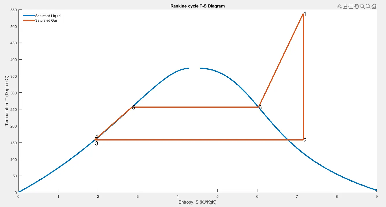
- Saturation curve is plotted in orangefor saturated liquid and saturated gas in T-S and in H-S it is black.
- Plot of T vs s and h vs s is created from all the points obtained from the program using the plot command and mentioning all the lables, linewidth, color and title.
- The plot changes as the user input changes for the above mentioned inputs .
- Results are displayed in the command window by using
fprintfcommand
COMMAND WINDOW WITH PLOT :
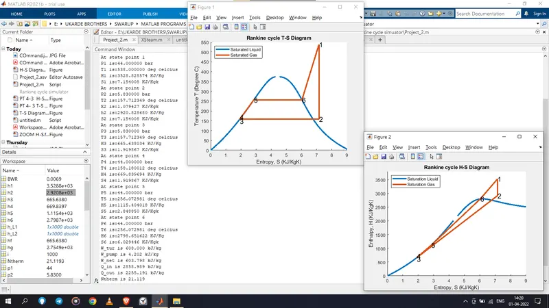
 RANKINE CYCLE
1-2 is Isentropic Expansion in the Turbine
2-3 is Constant Pressure Heat Rejection by the Condenser
3-4 is Isentropic Compression in the Pump (Pumping Process)
4-1 is Constant Pressure Heat Addition in Boiler
nValue of Pressure at Turbine Inlet, (in bar) =44
nValue of Temprature at Turbine Inlet, (in Degree Celcius) =538
nValue of Pressure at Condenser Inlet, (in bar) =5.83
Results
At state point 1
P1 is:44.000000 bar
T1 is:538.000000 deg celcius
H1 is:3528.828574 KJ/Kg
S1 is:7.154008 KJ/Kgk
At state point 2
P2 is:5.830000 bar
T2 is:157.712349 deg celcius
X2 is:1.079427 KJ/Kgk
h2 is:2920.828680 KJ/Kg
S2 is:7.154008 KJ/Kgk
At state point 3
P3 is:5.830000 bar
T3 is:157.712349 deg celcius
H3 is:665.638034 KJ/Kg
S3 is:1.919867 KJ/Kgk
At state point 4
P4 is:44.000000 bar
T4 is:158.180012 deg celcius
H4 is:669.839694 KJ/Kg
S4 is:1.919867 KJ/Kgk
At state point 5
P5 is:44.000000 bar
T5 is:256.072981 deg celcius
H5 is:1115.404018 KJ/Kg
S5 is:2.848850 KJ/Kgk
At state point 6
P6 is:44.000000 bar
T6 is:256.072981 deg celcius
H6 is:2798.651622 KJ/Kg
S6 is:6.029446 KJ/Kgk
W_tur is 608.000 kJ/kg
W_pump is 4.202 kJ/kg
W_net is 603.798 kJ/kg
Q_in is 2858.989 kJ/kg
Q_out is 2255.191 kJ/kg
Ntherm is 21.119
BWR is 0.007
S.S.C is 5.962
>>
RESULTS :
The performance of the Heat Engine was calculated and the following Observations were made:
Net work output : 603.798 kJ/kg
Thermal efficiency `ηtherm` = 21.119%
BWR = 0.007
S.S.C = 5.962
PLOTS T-S & H-S DIAGRAM
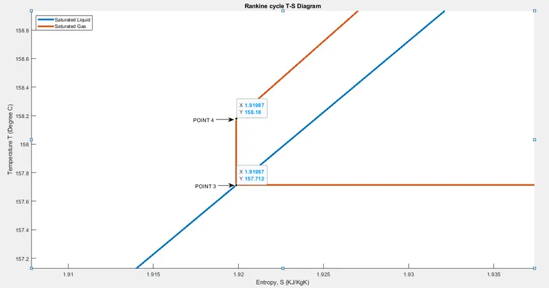
H-S DIAGRAM
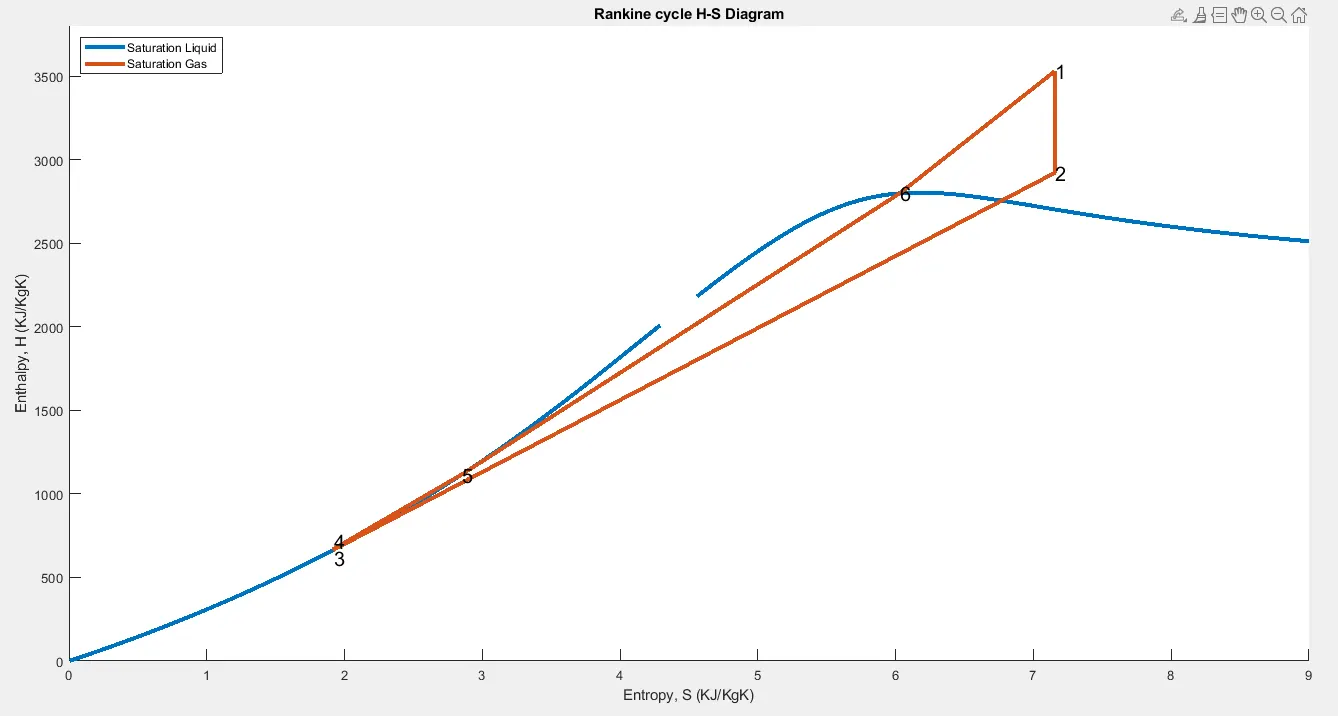
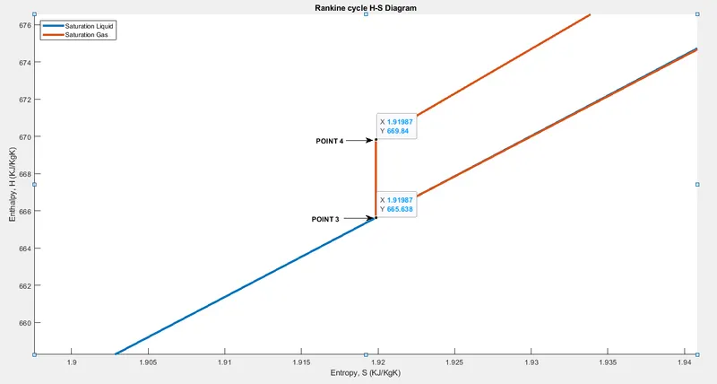
NO MAJOR ERROR FOUND
REFRENCE :
https://en.wikipedia.org/wiki/Rankine_cycle#Description
https://www.learnthermo.com/T1-tutorial/ch09/lesson-E/pg10.php