Week 4.1 - Genetic Algorithm

AIM:-

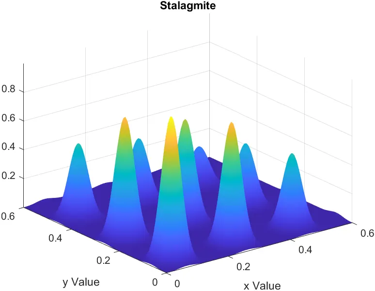
• Write a code in MATLAB to optimize the stalagmite function and find the global maxima of the function.
• Explain the concept of genetic algorithm in your own words and also explain the syntax for ga in MATLAB in your report.

INTRODUCTION:-

Genetic Algorithms(GAs) are adaptive heuristic search algorithms that belong to the larger part of evolutionary algorithms. Genetic algorithms are based on the ideas of natural selection and genetics. These are intelligent exploitation of random search provided with historical data to direct the search into the region of better performance in solution space. They are commonly used to generate high-quality solutions for optimization problems and search problems. Genetic algorithms simulate the process of natural selection which means those species who can adapt to changes in their environment are able to survive and reproduce and go to the next generation. In simple words, they simulate “survival of the fittest” among individuals of consecutive generations for solving a problem. Each generation consists of a population of individuals and each individual represents a point in search space and possible solution. Each individual is represented as a string of character/integer/float/bits. This string is analogous to the Chromosome.

Foundation of Genetic Algorithms

Genetic algorithms are based on an analogy with the genetic structure and behavior of chromosomes of the population. Following is the foundation of GAs based on this analogy –

1. Individuals in the population compete for resources and mate
2. Those individuals who are successful (fittest) then mate to create more offspring than others
3. Genes from the “fittest” parent propagate throughout the generation, that is sometimes parents create offspring which is better than either parent.
4. Thus each successive generation is more suited for their environment.

Five phases are considered in a genetic algorithm.

1. Initial population
2. Fitness function
3. Selection
4. Crossover
5. Mutation

Advantage of Genetic Algorithm(GA)

• The concept is easy to understand.
• GA search from a population of points, not a single point.
• GA uses payoff information, not derivatives.
• GA supports multi-objective optimization.
• GA is good for a "noisy" environment.
• GA is stochastic.
• Has very good parallel capabilities.

Disadvantage of Genetic Algorithm(GA)

• GA is computationally expensive(time-consuming).
• GA requires less information about the problem, but designing an objective function and getting the representation and operator right can be difficult.
• Useful when the search space is very large and there are a large number of parameters involved.

Application of Genetic Algorithm(GA)

• Optimization − Genetic Algorithms are most commonly used in optimization problems wherein we have to maximize or minimize a given objective function value under a given set of constraints. The approach to solve Optimization problems has been highlighted throughout the tutorial.

• Economics − GAs are also used to characterize various economic models like the cobweb model, game theory equilibrium resolution, asset pricing, etc.

• Neural Networks − GAs are also used to train neural networks, particularly recurrent neural networks.

• Parallelization − GAs also have very good parallel capabilities and prove to be very effective means in solving certain problems, and also provide a good area for research.

• Image Processing − GAs are used for various digital image processing (DIP) tasks as well as dense pixel matching.

• Vehicle routing problems − With multiple soft time windows, multiple depots, and a heterogeneous fleet.

• Scheduling applications − GAs are used to solve various scheduling problems as well, particularly the timetabling problem.

• Machine Learning − as already discussed, genetics-based machine learning (GBML) is a niche area in machine learning.

• Robot Trajectory Generation − GAs have been used to plan the path that a robot arm takes by moving from one point to another.

• Parametric Design of Aircraft − GAs have been used to design aircraft by varying the parameters and evolving better solutions.

• DNA Analysis − GAs have been used to determine the structure of DNA using spectrometric data about the sample.

• Multimodal Optimization − GAs are obviously very good approaches for multimodal optimization in which we have to find multiple optimum solutions.

• Traveling salesman problem and its applications − GAs have been used to solve the TSP, which is a well-known combinatorial problem using novel crossover and packing strategies.

Syntax of GA function

x = ga(fun,nvars)

x = ga(fun,nvars,A,b)

x = ga(fun,nvars,A,b,Aeq,beq)

x = ga(fun,nvars,A,b,Aeq,beq,lb,ub)

x = ga(fun,nvars,A,b,Aeq,beq,lb,ub,nonlcon)

x = ga(fun,nvars,A,b,Aeq,beq,lb,ub,nonlcon,options)

x = ga(fun,nvars,A,b,Aeq,beq,lb,ub,nonlcon,intcon)

x = ga(fun,nvars,A,b,Aeq,beq,lb,ub,nonlcon,intcon,options)

x = ga(problem)

[x,fval] = ga(___)

[x,fval,exitflag,output] = ga(___)

[x,fval,exitflag,output,population,scores] = ga(___)

Explaination of GA syntax:-

• x = ga(fun,nvars) finds a local unconstrained minimum, x, to the objective function, fun. nvars is the dimension (number of design variables) of fun.
• x = ga(fun,nvars,A,b) finds a local minimum x to fun, subject to the linear inequalities A*x ≤ b. ga evaluates the matrix product A*x as if x is transposed (A*x').
• x = ga(fun,nvars,A,b,Aeq,beq) finds a local minimum x to fun, subject to the linear equalities Aeq*x = beq and A*x ≤ b. (Set A=[] and b=[] if no linear inequalities exist.) ga evaluates the matrix product Aeq*x as if x is transposed (Aeq*x').
• x = ga(fun,nvars,A,b,Aeq,beq,lb,ub) defines a set of lower and upper bounds on the design variables, x, so that a solution is found in the range lb ≤ x ≤ ub. (Set Aeq=[] and beq=[] if no linear equalities exist.)
• x = ga(fun,nvars,A,b,Aeq,beq,lb,ub,nonlcon) subjects the minimization to the constraints defined in nonlcon. The function nonlcon accepts x and returns vectors C and Ceq, representing the nonlinear inequalities and equalities respectively. ga minimizes the fun such that C(x) ≤ 0 and Ceq(x) = 0. (Set lb=[] and ub=[] if no bounds exist.)
• x = ga(fun,nvars,A,b,Aeq,beq,lb,ub,nonlcon,options) minimizes with the default optimization parameters replaced by values in options. (Set nonlcon=[] if no nonlinear constraints exist.) Create options using optimoptions.
• x = ga(fun,nvars,A,b,Aeq,beq,lb,ub,nonlcon,options,intcon) or x = ga(fun,nvars,A,b,Aeq,beq,lb,ub,nonlcon,intcon,options) requires that the variables listed in intcon take integer values.
• x = ga(problem) finds the minimum for problem, a structure described in problem.
• [x,fval] = ga(___), for any previous input arguments, also returns fval, the value of the fitness function at x.
• [x,fval,exitflag,output] = ga(___) also returns exitflag, an integer identifying the reason the algorithm terminated, and output, a structure that contains output from each generation and other information about the performance of the algorithm.
• [x,fval,exitflag,output,population,scores] = ga(___) also returns a matrix population, whose rows are the final population, and a vector scores, the scores of the final population.

MATLAB code for Genetic algorithm:-

%Degfinig our search space
x = linspace(0,0.6,150);
y = linspace(0,0.6,150);

%Creating a 2dimentional mesh
[xx,yy] = meshgrid(x,y);
%Evaluating the stalagmite functiontion
for i=1:length(xx)
    for j=1:length(yy)
input_vector(1)=xx(i,j);
input_vector(2)=yy(i,j);
f(i,j)=stalagmite_function(input_vector);
    end
end

figure(1)
surfc(xx,yy,-f)
shading interp
xlabel('x Value')
ylabel('y Value')
title('Stalagmite')

%study 1
n_iteration = 50;
tic
for i = 1:n_iteration
[inputs,fopt(i)] = ga(@stalagmite_function,2);
xopt1(i) = inputs(1);
yopt1(i) = inputs(2);
end
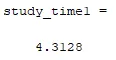
study_time1 = toc

%plotting
figure(2)
subplot(2,1,1)
hold on
surfc(x,y,-f)
title('Unbounded Input')
xlabel('x Value')
ylabel('y Value')
shading interp
hold on
plot3(xopt1,yopt1,-fopt,'marker','o','markersize',4,'markerfacecolor','r')
subplot(2,1,2)
plot(-fopt)
xlabel('Iteration')
ylabel('Function minimum')
tic

%study2 - statistical behaviour with upper and lower bounds
for i=1:n_iteration
[inputs,fopt(i)] = ga(@stalagmite_function,2,[],[],[],[],[0;0],[0.6;0.6]);
xopt(i) = inputs(1);
yopt(i) = inputs(2);
end
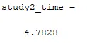
study2_time=toc

%plotting
figure(3)
subplot(2,1,1)
surfc(x,y,-f)
shading interp
title('Bounded Inputs')
xlabel('x Value')
ylabel('y Value')
hold on
plot3(xopt,yopt,-fopt,'marker','o','markersize',4,'markerfacecolor','r')
subplot(2,1,2)
plot(-fopt)
xlabel('Iteration')
ylabel('Function minimum')

%study3 increasing the population size
options = optimoptions(@ga);
options = optimoptions(@ga,'populationsize',500);
tic
for i=1:n_iteration
[inputs,fopt(i)]=ga(@stalagmite_function,2,[],[],[],[],[0;0],[0.6;0.6],[],[],options);
xopt(i)=inputs(1);
yopt(i)=inputs(2);
end

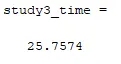
study3_time=toc

figure(4)
subplot(2,1,1)
surfc(x,y,-f)
shading interp
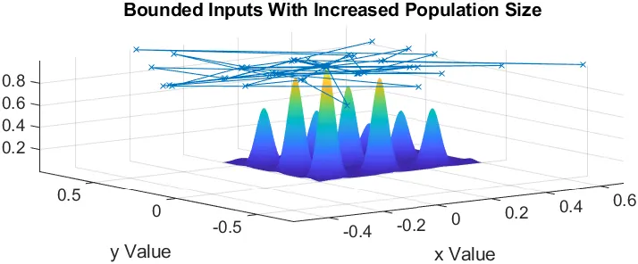
title('Bounded Inputs With Increased Population Size')
xlabel('x Value')
ylabel('y Value')
hold on
plot3(xopt1,yopt1,-fopt,'marker','x','markersize',4,'markerfacecolor','k')
subplot(2,1,2)
plot(-fopt)
xlabel('Iteration')
ylabel('Function minimum')

MATLAB code for stalagmite function:-

function [f] = stalagmite_function(input_vector)
x1 = input_vector(1);
y1 = input_vector(2);
f1x = (sin(5.1*pi*x1+0.5))^6;
f1y = (sin(5.1*pi*y1+0.5))^6;
f2x = exp(-4*log(2)*((x1-0.0667).^2)/0.64);
f2y = exp(-4*log(2)*((y1-0.0667).^2)/0.64);
f = -(f1x*f1y*f2x*f2y);
end

OUTPUT:-

• Stalagmite function

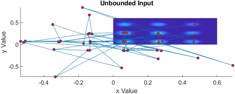
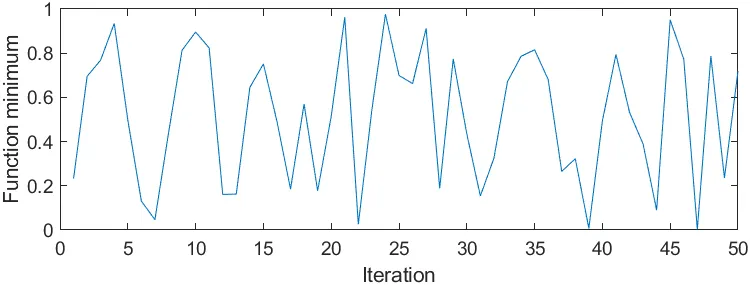
• Unbounded input

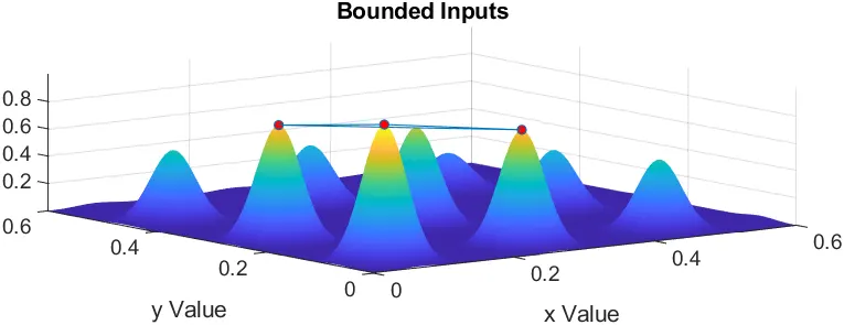
• Bounded input

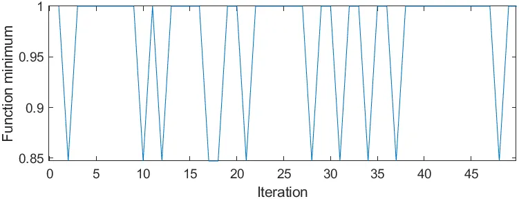
• Bounded input with increased population size