Week 4.1 - Genetic Algorithm
Aim-Write a code in MATLAB to optimise the stalagmite function and find the global maxima of the function.
Introduction to genetic algorithms-
Genetic algorithms are a type of optimization algorithm, meaning they are used to find the maximum or minimum of a function. In this paper, we introduce, illustrate, and discuss genetic algorithms for beginning users. We show what components make up genetic algorithms and how to write them. Using MATLAB, we program several examples, including a genetic algorithm that solves the classic Traveling Salesman Problem. We also discuss the history of genetic algorithms, current applications, and future developments. Genetic algorithms are a type of optimization algorithem.
Introduction to optimization-
In the optimization of a design, the design objective could be simply to minimize the cost of production or to maximize the efficiency of production. An optimization algorithm is a procedure that is executed iteratively by comparing various solutions till an optimum or satisfactory solution is found. With the advent of computers, optimization has become a part of computer-aided design activities. There are two distinct types of optimization algorithms widely used today.
The genetic algorithm solves both constrained and unconstrained optimization problems based on natural selection, which drives biological evolution. The genetic algorithm repeatedly modifies a population of individual solutions. At each step, the genetic algorithm selects individuals at random from the current population to be parents and uses them to produce the children for the next generation. Over successive generations, the population "evolves" toward an optimal solution. You can apply the genetic algorithm to solve a variety of optimization problems that are not well suited for standard optimization algorithms, including problems in which the objective function is discontinuous, nondifferentiable, stochastic or highly nonlinear. The genetic algorithm can address mixed integer programming problems, where some components are restricted to integer-valued.
The genetic algorithm uses three main types of rules at each step to create the next generation from the current population
-
Selection rules select the individuals, called parents, who contribute to the next generation's population.
-
Crossover rules combine two parents to form children for the next generation.
-
Mutation rules apply random changes to individual parents to form children.
The genetic algorithm differs from a classical, derivative-based, optimization algorithm in two main ways, as below
Classical Algorithm
- Generates a single point at each iteration. The sequence of points approaches an optimal solution.
- Selects the next point in the sequence by a deterministic computation.
Genetic Algorithm
- Generates a population of points at each iteration. The best point in the population approaches an optimal solution
- Selects the next population by computation which uses random number generators.
The following outline summarizes how the genetic algorithm works:
-
The algorithm begins by creating a random initial population.
-
The algorithm then creates a sequence of new populations. At each step, the algorithm uses the individuals in the current generation to create the next population. To create a new population.
the algorithm performs the following steps
-
Scores each member of the current population by computing its fitness value. These values are called the raw fitness scores.
-
Scales the raw fitness scores to convert them into a more usable range of values. These scaled values are called expectation values.
-
Selects members, called parents, based on their expectations.
-
Some of the individuals in the current population that have lower fitness are chosen as elite. These elite individuals are passed to the next population.
-
Produces children from the parents. Children are produced either by making random changes to a single parent mutation or by combining the vector entries of a pair of parents crossover.
-
Replaces the current population with the children to form the next generation.
-
-
The algorithm stops when one of the stopping criteria is met.
-
The algorithm takes modified steps for linear and integer constraints.
-
The algorithm is further modified for nonlinear constraints.
Syntax
Description
x = ga(fun,nvars,A,b,Aeq,beq,lb,ub,nonlcon)nonlcon. The function nonlcon accepts x and returns vectors C and Ceq, representing the nonlinear inequalities and equalities respectively. ga minimizes the fun such that C(x) ≤ 0 and Ceq(x) = 0. (Set lb=[] and ub=[] if no bounds exist.)
x = ga(fun,nvars,A,b,Aeq,beq,lb,ub,nonlcon,intcon)x = ga(fun,nvars,A,b,Aeq,beq,lb,ub,nonlcon,intcon,options)intcon take integer values.
writing of a Function code
function f = stalagmite_1(input_vector)
x1 = input_vector(1);
y1 = input_vector(2);
f1 = (sin((5.1*pi*x1)+0.5)).^6;
f2 = (sin((5.1*pi*y1)+0.5)).^6;
f3 = exp((-4*(log(2))*(x1-0.0667).^2)/0.64);
f4 = exp((-4*(log(2))*(y1-0.0667).^2)/0.64);
f = -(f1.*f2.*f3.*f4)
end
explanation coding
- at first, we have to use the word Function to start the function command
- and then we want to create a templet and this is a code templet and name for the templet
- we are going to name the code templet stalagmite_1
- we are going to use this formula to solve the equation.
- so whenever we want to substitute different values we just call this function and then pass in the right values
- then we have to save the function while saving the name of the function and the name of the file should exactly be the same
- the calling the function means using the function and using the templates with the appropriate values
- we have to ensure the no of inputs we provide match the orders of inputs also match
- end word is used to end the function command.
writing of Code
clear all
close all
clc

x = linspace(0,0.6,150);
y = linspace(0,0.6,150);

num_cases = 50


% Creating a 2Dimensional mesh
[xx,yy] = meshgrid(x,y)


% Logic
for i = 1:length(xx)
for j = 1:length(yy)
input_vector(1) = xx(i,j)
input_vector(2) = yy(i,j)
f(i,j) = stalagmite_1(input_vector)
end
end
 tic
% Study 1 - Satistical behaviour
for i = 1:num_cases
    [inputs, fopt(i)] = ga(@stalagmite_1, 2);
    xopt(i) = inputs(1);
    yopt(i) = inputs(2);
end

study_time = toc

figure(1)
subplot(2,1,1)
hold on
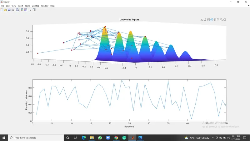
surfc(x, y, -f)
shading interp
plot3(xopt,yopt,-fopt,'marker','o','markersize',5,'markerfacecolor','r')
title('Unbonded inputs')
subplot(2,1,2)
plot(-fopt)
xlabel('Iterations')
ylabel('Function minimum')

tic
% Study 2 - Stastical behaviour - with upper & lower bounds
for i = 1:num_cases
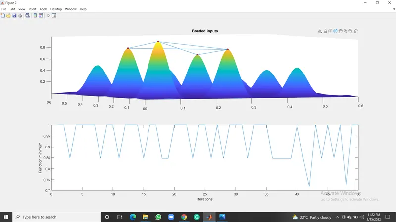
    [inputs, fopt(i)] = ga(@stalagmite_1,2,[],[],[],[],[0;0],[0.6;0.6]);
    xopt(i) = inputs(1);
    yopt(i) = inputs(2);
end
study2_time = toc

figure(2)
subplot(2,1,1)
hold on
surfc(x, y, -f)
shading interp
plot3(xopt,yopt,-fopt,'marker','o','markersize',5,'markerfacecolor','r')
title('Bonded inputs')
subplot(2,1,2)
plot(-fopt)
xlabel('Iterations')
ylabel('Function minimum')

% Study 3 increaing GA iterations
options = optimoptions('ga');
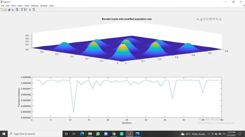
options = optimoptions(options,'PopulationSize', 170);


tic
for i = 1:num_cases
    [inputs, fopt(i)] = ga(@stalagmite_1,2,[],[],[],[],[0;0],[0.6;0.6],[],[],options);
    xopt(i) = inputs(1);
    yopt(i) = inputs(2);
end

study3_time = toc
figure(3)
subplot(2,1,1)
hold on
surfc(x, y, -f)
shading interp
plot3(xopt,yopt,-fopt,'marker','o','markersize',5,'markerfacecolor','r')
title('Bonded inputs with modified population size')
subplot(2,1,2)
plot(-fopt)
xlabel('Iterations')
ylabel('Function minimum')
explanation of code-
- to get started we have to open a new file
- whenever we start a new program it is good practice to include some commands
- input variables are taken
- linspace command is used to get 150 values between the 0and0.6 they are in 1d
- meshgrid command is used to covert 1d into 2d
- we have to ensure the no of inputs we provide match the orders of inputs also match
- we have to ensure that both the function program and the working program must be in the same folder
- we have to use the surfc command is used to create a graph
- shading interp is used to get the smooth surface
- and the output is displayed as given below
Output
Unbonded inputs
Bonded inputs
Bonded inputs with modified population size
research resources