Week 4.1 - Genetic Algorithm

OBJECTIVE:

Write a program to optimize the stalagmite function and find the global maxima of the function.

PRE-REQUISITES:

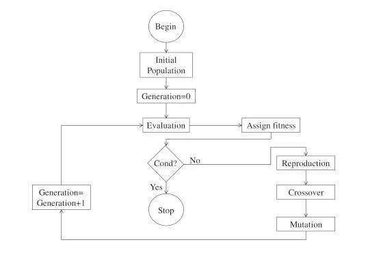
i) Genetic algorithms are randomized search algorithms that have been developed in an effort to imitate the mechanics of natural selection and natural genetics.

ii) Genetic algorithms operate on string structures, like biological structures, which are evolving in time according to the rule of survival of the fittest by using a randomized yet structured information exchange.

iii) Thus, in every generation, a new set of strings is created, using parts of the fittest members of the old set.

iv) The main characteristics of a genetic algorithm are as follows:

a) The genetic algorithm works with the coding of a parameter set, not the parameters themselves.

b) The genetic algorithm initiates its search from a population of points, not a single point.

PROCEDURE:

a) Main Code:

clear all
close all
clc

%Defining search space
x = linspace(0,0.6,500);
y = linspace(0,0.6,500);

%Defining number of cases
num_cases = 50

%Creating a two-dimensional mesh
[xx yy] = meshgrid(x,y);

%Evaluating the stalagmite function
for i = 1:length(xx)
    for j = 1:length(yy)
        input_value(1) = xx(i,j);
        input_value(2) = yy(i,j);
        f(i,j) = stalagmite(input_value);
    end
end

%Study 1: Unbounded statistical behaviour
tic
for l = 1:num_cases
    [inputs1,fopt1(l)] = ga(@stalagmite,2);
    xopt1(l) = inputs1(1);
    yopt1(l) = inputs1(2);
end

%Calculating run-time
study_time1 = toc

%Plotting
figure(1)
subplot(2,1,1)
hold on 
surfc(xx,yy,-f)
shading interp
plot3(xopt1,yopt1,-fopt1)
subplot(2,1,2)
plot(-fopt1)

%Study 2: Statistical behaviour using upper and lower bounds
tic
for m = 1:num_cases
    [inputs2,fopt2(m)] = ga(@stalagmite,2,[],[],[],[],[0;0],[0.6;0.6]);
    xopt2(m) = inputs2(1);
    yopt2(m) = inputs2(2);
end

%Calculating run-time
study_time2 = toc

%Plotting
figure(2)
subplot(2,1,1)
hold on 
surfc(xx,yy,-f)
shading interp
plot3(xopt2,yopt2,-fopt2)
subplot(2,1,2)
plot(-fopt2)

%Study 3: Statistical behaviour using upper and lower bounds
options = optimoptions('ga');
options = optimoptions(options, 'populationsize', 350);
tic
for n = 1:num_cases
    [inputs3,fopt3(n)] = ga(@stalagmite,2,[],[],[],[],[0;0],[0.6;0.6],[],[],options);
    xopt3(n) = inputs3(1);
    yopt3(n) = inputs3(2);
end

%Calculating run-time
study_time3 = toc

%Plotting
figure(3)
subplot(2,1,1)
hold on 
surfc(xx,yy,-f)
shading interp
plot3(xopt3,yopt3,-fopt3)
subplot(2,1,2)
plot(-fopt3)

b) Steps involved:

i) Using the linspace command x and y variables are defined ranging from 0 to 0.6 in 150 elements.

ii) Use the meshgrid command to generate a 2-dimensional mesh plane.

iii) For evaluating the stalagmite function two for loops are used, the values for two input variables are given by the 2-dimensional mesh plane generated with the help of meshgrid command.

iv) Now starting with the first study that is unbounded statistical behavior.

v) Here for defining the number of iterations a variable 'num_cases' is used and is set to 50.

vi) For determining the time taken by the code to evaluate, tic and toc command is used.

vii) The format of 'ga' (genetic algorithm) used in this case is “ [inputs , fopt] = ga (fun , nvars)“.

viii) For plotting the graphs, the figure command is used for a new figure window, subplot is used for dividing the window into parts, and here it divides the figure window into two parts.

ix) In the first half two graphs are plotted in a single graph using the hold on command, surfc command is used which plots a surface graph and the other graph is a 3-dimensional line plot for this the command used is plot3.

x) X and Y label is given along with the title.

xi) The second study is statistical behavior with upper and lower bound.

xii) Here for defining the number of iterations a variable 'num_cases' is used and is set to 50.

xiii) The format of 'ga' (genetic algorithm) used in this case is “ [inputs , fopt] = ga (fun,nvars,A,b,Aeq,beq,lb,ub).

xiv) Now for plotting the graphs, figure command is used for a new figure window, subplot is used for dividing the window into parts, and here it divides the figure window into two parts.

xv) In the first half two graphs are plotted in a single graph using the “hold on” command, surfc command is used which plots a surface graph and the other graph is a 3-dimensional line plot for this the command used is plot3.

xvi) X and Y label is given along with the title.

xvii) The third study is statistical behavior with increased population size.

xviii) Here for defining the number of iterations a variable “num_cases” is used and is set to 50.

xix) The format of 'ga' (genetic algorithm) used in this case is “ [inputs,fopt]=ga(fun,nvars,A,b,Aeq,beq,lb,ub,nonlcon,IntCon,options).

xx) For plotting the graphs, the figure command is used for a new figure window, subplot is used for dividing the window into parts, and here it divides the figure window into two parts.

xxi) In the first half two graphs are plotted in a single graph using the hold on command, surfc command is used which plots a surface graph and the other graph is a 3-dimensional line plot for this the command used is plot3.

xxii) X and Y label is given along with the title.

xxiii) Now for printing the data on the command window “fprintf” command is used.

c) Stalagmite function:

function [f] = stalagmite(input)
x = input(1);
y = input(2);

f1_x = (sin((5.1*pi*x) + 0.5))^6;
f1_y = (sin((5.1*pi*y) + 0.5))^6;

f2_x = exp(-4*log(2)*((x - 0.0667)^2)/0.64);
f2_y = exp(-4*log(2)*((y - 0.0667)^2)/0.64);

f = -(f1_x*f1_y*f2_x*f2_y);

end

d) Steps involved:

i) For the function code the function is created and its input vector is specified.

ii) Then all the four equations are written with the inputs from the meshgrid.

iii) Now for maximizing the function a negative sign is used.

RESULT:

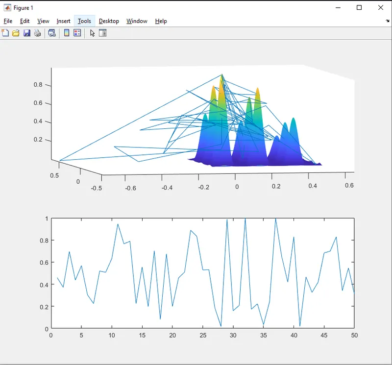
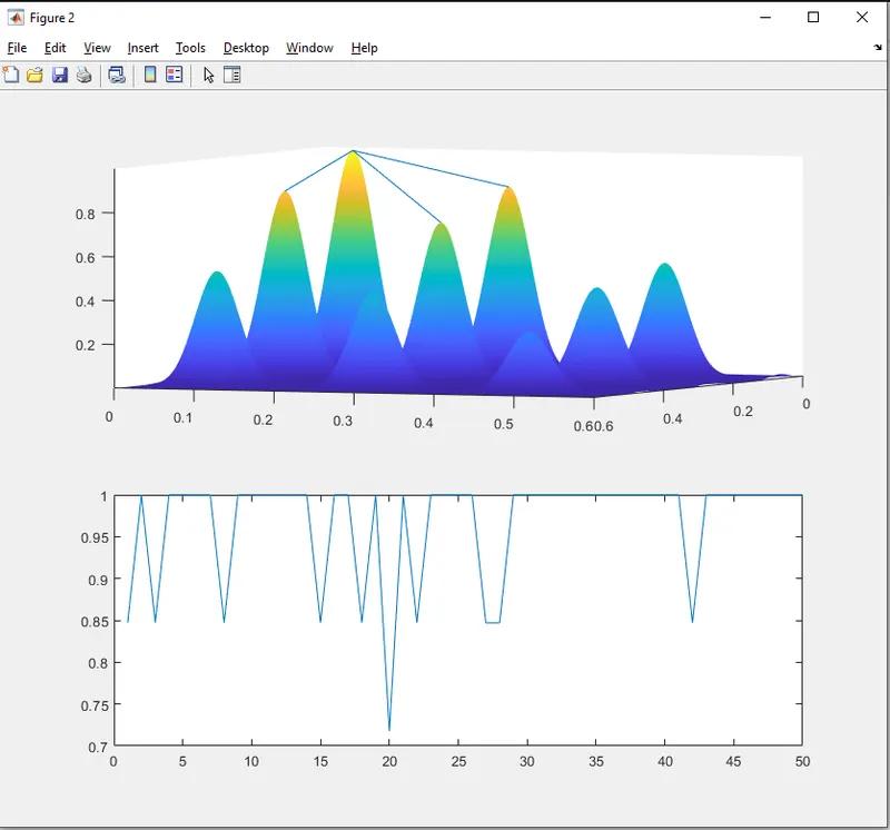
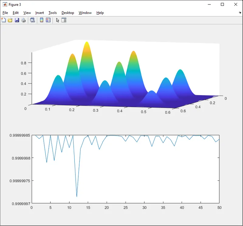
i) The following tables shows the plots obtained for all the cases:

SL No.	Case	2-D Plot	3-D Plot
1.	Unbounded Statistical Behavior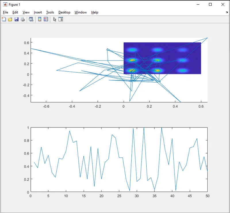
2.	Statistical Behavior with upper and lower bound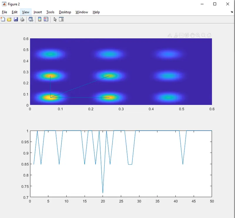
3.	Statistical Behavior with increased population size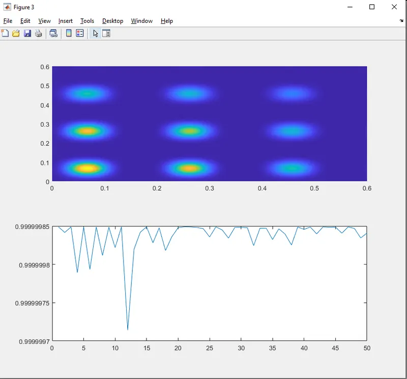

ii) The following table shows the run-time for all the cases:

SL No.	Case	Study Time(s)
1	Unbounded Statistical Behavior	4.39
2	Statistical Behavior with upper and lower bound	6.45
3	Statistical Behavior with increased population size	29.15

iii) The global maxima is nearly 1 for the given stalagmite function.

CONCLUSION:

i) Studied the genetic algorithm and stalagmite function.

ii) Compared the different cases and documented the changes.