TO UNDERSTAND THE CONCEPT OF GENETIC ALGORITHM AND TO OTIMIZE THE STALAGMITE FUNCTION TO FIND THE GLOBAL MAXIMA OF A FUNCTION.

AIM:

1. TO UNDERSTAND THE CONCEPT OF GENETIC ALGORITHM
2. EXPLAINING THE SYNTAX OF GA
3. TO OTIMIZE THE STALAGMITE FUNCTION TO FIND THE GLOBAL MAXIMA OF A FUNCTION.
4. PLOT GRAPH OF 3 STUDIES AND FOR F MAXIMUM VS NUMBER OF ITERATIONS.

INTRODUCTION:

DEFINITION OF GA:-

In computer science and operation research, a genetic algorithm (GA) is a process inspired by the process of natural selection that belongs to the larger class of evolutionery algorithms (EA). Genetic algorithms are commonly used to generate high-quality solutions to optimization and search problems by relying on biologically inspired operators such as mutation, crossover and selection. Some examples of GA applications include optimizing decesion trees for better performance.

Genetic Algorithms are a search based operations based on the cconcept of natural selection and genetics. GA is a part of a bigger function known as EVOLUTIONARY COMPUTATION.

In GA we have a pool or a population of possible solutions to a given problem. These population then undergo process like reecombination and genetic mutation reproducing newer offsprings and the similar process goes on for several generations untill we reach a stopping criteria.

The each offspring produced have a 'fitness value'. And the fiiter individual produced via genetic mutation and reproduction is then considered to mate producing new offsprings.Thus we keep evolving to newer and more fitter individual untill the stopping criteria.

Advantages of GA:

GA has many advantages.

• does not require derivative information.
• very fast and efficient
• produces list of solutions('good') not just a single solution
• it is very useful when the search space is large and there are number of parameters involved
• very reliable as it produces solution almost every time and it gets better every time.
• it has very good parallel capabilities
• works well on discrete/continous problem
• supports multi-objective optimization.

Disadvantages of GA:

• expensive and time consuming
• not suited for problems which do not have derivatiive information
• cannot converge into optimal solution if not implemented properly.

STEPS INVOLVED TO SOLVE GA:

• Initial population
• Fitness function
• Selection
• Crossover
• Mutation

PROCESS OF NATURAL SELECTION:

The process of natural selection starts with the selection of fittest individuals from a population. They produce offspring which inherit the characteristics of the parents and will be added to the next generation. If parents have better fitness, their offspring will be better than parents and have a better chance at surviving. This process keeps on iterating and at the end, a generation with the fittest individuals will be found.

This notion can be applied for a search problem. We consider a set of solutions for a problem and select the set of best ones out of them.

DEFINING ALL THE FIVE PROCESSESS:

INITIAL POPULATION:

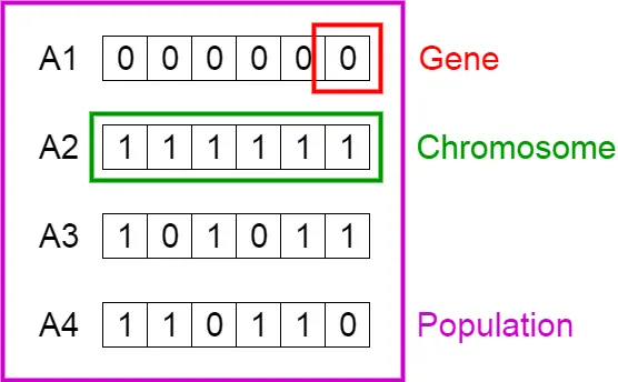
The process begins with a set of individuals which is called a Population. Each individual is a solution to the problem you want to solve.

An individual is characterized by a set of parameters (variables) known as Genes. Genes are joined into a string to form a Chromosome (solution).

In a genetic algorithm, the set of genes of an individual is represented using a string, in terms of an alphabet. Usually, binary values are used (string of 1s and 0s). We say that we encode the genes in a chromosome.

FITNESS FUNCTION

The fitness function determines how fit an individual is (the ability of an individual to compete with other individuals). It gives a fitness score to each individual. The probability that an individual will be selected for reproduction is based on its fitness score.

SELECTION:

The idea of selection phase is to select the fittest individuals and let them pass their genes to the next generation.

Two pairs of individuals (parents) are selected based on their fitness scores. Individuals with high fitness have more chance to be selected for reproduction.

CROSSOVER:

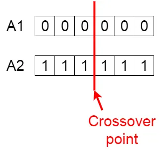
Crossover is the most significant phase in a genetic algorithm. For each pair of parents to be mated, a crossover point is chosen at random from within the genes.

For example, consider the crossover point to be 3 as shown below.

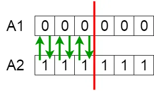
Offspring are created by exchanging the genes of parents among themselves until the crossover point is reached.

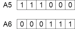
The new offspring are added to the population.

MUTATION:

In certain new offspring formed, some of their genes can be subjected to a mutation with a low random probability. This implies that some of the bits in the bit string can be flipped.

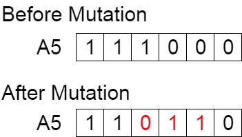
MUTATION OCCURS TO MAITAIN DIVERSITY AND WITHIN THE POPULATION AND PREVENT PREMATURE CONVERGENCE.

EXPLANATIONS OF THE COMMANDS USED IN THIS PROGRAMME:

X = ga(fun,nvars,A,b,Aeq,beq,lb,ub,nonlcon,options)

ga = inbuilt function of MATLAB used to find minimum values of a function

fun = function handle

nvars = number of variables used in this programme(x,y)

A,b = linear inequality constraints

Aeq,beq = linear equality constraints

lb = lower bound

ub = upper bound

nonlcon = non linear constraints

options = optimization options

options = optimoptions(prob,name,value)

prob = optimazation problem

name = argument name

value = corresponding value

[]= represents non existent conditions

subplot(m,n,position)

m = row

n = coloumn

position = the respective positioning

FUNCTION FOR STALAGMITE

function [f] = stalagmite(input)
x = input(1);
y = input(2);

f1_x = (sin((5.1*pi*x)+0.5)).^6;
f1_y = (sin((5.1*pi*y)+0.5)).^6;
f2_x = exp(-4*log(2)*((x-0.0667).^2)/0.64);
f2_y = exp(-4*log(2)*((y-0.0667).^2)/0.64);
%to determine global maxima
f = -(f1_x.*f1_y.*f2_x.*f2_y);
end

EXPLANATION OF THE CODE:

THE STALAGMITE FUNCTION IS GIVEN BY:

`f = -(f1_x.*f1_y.*f2_x.*f2_y)`

HERE IN THIS FUNCTION THE "(-)NEGEATIVE SIGN)" IS TO FIND THE GLOBAL MAXIMA `f = -(f1_x.*f1_y.*f2_x.*f2_y)`

PROGRAMME TO FIND THE GLOBAL MAXIMA:

clear all 
close all
clc

%defining search space
x = linspace(0,0.6,150)
y = linspace(0,0.6,150)
num_cases = 50;
%creating 2D mesh
[xx,yy] = meshgrid(x,y);
for i = 1:length(xx)
    for j = 1:length(yy)
        input(1) = xx(i,j);
        input(2) = yy(i,j);
      f(i,j)= stalagmite(input); 
    end
end
%study1- statistical behaviour
tic
for l = 1:num_cases
    [input1, fopt1(l)] = ga(@stalagmite,2);
    xopt1(l) = input1(1);
    yopt1(l) = input1(2);
end
%to measure the time taken
study1_time = toc;
figure(1)
subplot(2,1,1) %2 PLOTS IN 2 ROWS AND 1 COLOUMN AND THE 1ST POSITION
hold on
surf(x,y,f)
shading interp %TO ELIMINATE GRID LINES
plot3(xopt1,yopt1,fopt1,'marker','o','MarkerSize',6,'MarkerFaceColor','r')
title('outbound inputs')
subplot(2,1,2)
plot(fopt1)
xlabel('iterations')
ylabel('function maximum')

%study2-statistical behavour using upper and lower bound
tic
for m = 1:num_cases
    [input2,fopt2(m)] = ga(@stalagmite,2,[],[],[],[],[0;0],[1;1]);
    xopt2(m) = input2(1);
    yopt2(m) = input2(2);
end
study2_time = toc;
figure(2)
subplot(2,1,1) %2 PLOTS IN 2 ROWS AND 1 COLOUMN AND THE 1ST POSITION
hold on
surf(x,y,f)
shading interp %TO ELIMINATE GRID LINES
plot3(xopt2,yopt2,fopt2,'marker','o','MarkerSize',6,'MarkerFaceColor','r')
title('outbound inputs')
subplot(2,1,2)
plot(fopt2)
xlabel('iterations')
ylabel('function maximum')

%study3-statistical behaviour of upper bound and lower bound and increasing
%the size 
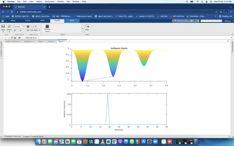
options = optimoptions('ga','populationsize',350)
tic
for n = 1:num_cases
    [input3,fopt3(n)] = ga(@stalagmite,2,[],[],[],[],[0;0],[1;1],[],[],options);
    xopt3(n) = input3(1);
    yopt3(n) = input3(2);
end
study3_time = toc;
figure(3)
subplot(2,1,1) %2 PLOTS IN 2 ROWS AND 1 COLOUMN AND THE 1ST POSITION
hold on
surf(x,y,f)
shading interp %TO ELIMINATE GRID LINES
plot3(xopt3,yopt3,fopt3,'marker','o','MarkerSize',6,'MarkerFaceColor','r')
title('outbound inputs')
subplot(2,1,2)
plot(fopt3)
xlabel('iterations')
ylabel('function maximum')

EXPLANATION FOR THE PROGRAMME AND STEPS:

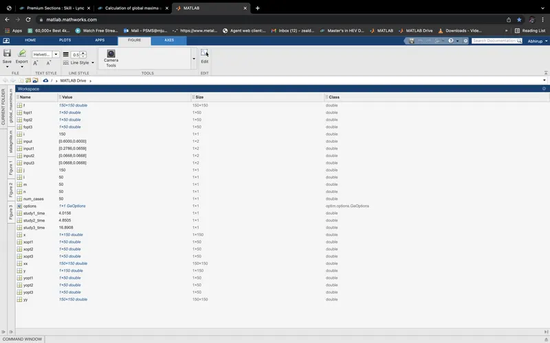
• The search is defined for x and y by giving linspace command with 150 intervals between 0 and 0.6
• the number of iterations is given to 50
• the 2D meshgrid is stored in f(i,j) and the meshgrid is created by using meshgrid command

%STUDY 1 - statistical behaviour:

To get the values of x and y we have given the iterations to the for loop of 50 and defined the number of variables as 2 and called the "stalagmite" function.

• surf command is used to get the 3D plot
• shading interp command is used to get rid of the grid lines
• these values are then plotted by the command plot3 to get a 3D plot
• tic and toc command is used to get the amount of time consumed to arrive at the solution
• subplot command is used to plot both the curves

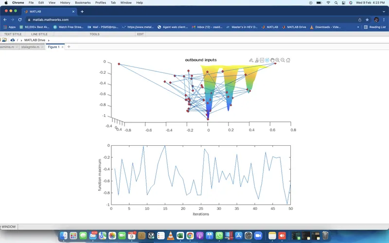
Result:

we can see from the above plot that the values are scattered.

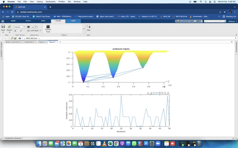
%Step2 -statistical behavour using upper and lower bound

Same steps have been follwed in this study except for a small change

[input2,fopt2(m)] = ga(@stalagmite,2,[],[],[],[],[0;0],[1;1]);

the above study used to bound the values within a range to provide more accurate results.also this study uses the syntax with the definition of lower bound and upper bound values in the form of x and y i.e. [0;0],[1;1] respectively and [] represents to the inequalities and equalitites pertaining to the function does not exist.

Results:

we can see that the values are now comparatively less scattered than %study1

%study3-statistical behaviour of upper bound and lower bound and increasing the size

In this study we are increasing the population size and reastricting search space which will ultimately provide us the best possible solution for global maxima of the function unlike the previous 2 cases.

[input3,fopt3(n)] = ga(@stalagmite,2,[],[],[],[],[0;0],[1;1],[],[],options);

so the above command is used and the values are then plotted which provides us with the global maxima as required.

WORKSPACE DETAILS FOR THE VALUES

CONCULSION: THUS THE GOLBAL MAXIMA IS ACHEIVED

NOTE: NO ERRORS FACED

MATERIALS USED FOR HELP:

• WIKIPEDIA
• YOUTUBE
• https://electricalvoice.com/genetic-algorithm-advantages-disadvantages/
• https://towardsdatascience.com/introduction-to-genetic-algorithms-including-example-code-e396e98d8bf3
• https://www.tutorialspoint.com/genetic_algorithms/genetic_algorithms_introduction.htm

THESE MATERIALS ARE USED FOR IDEA AND REASEARCH .