GENETIC ALGORITHM

Genetic Algorithm

Genetic Algorithms or GAs are basically a set of search algorithms that runs based on Charles Darwin’s ‘Theory of Natural Selection’. A common use of GAs is to generate high quality solutions for search and optimization problems.

Natural selection basically means that the species which can adapt to the changes in the environment will be able to survive and reproduce thereby going to the next generation. Or simply put , the fittest will survive. So the GAs work based on this idea. The GAs simulate the fittlest solution among the bunch of solutions or we can call it generations from solving the problem. Every single generation has a separate population of individuals and each individual represents a point in the search space and its solution.

How GAs work ?

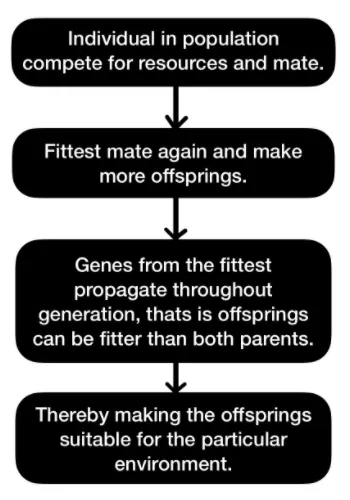
The basic foundation of the working GAs are in sync with the genetic structure and the behavior of chromosomes of the population. The flow chart below shows the foundation of GAs.

Search spaces

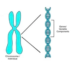
The GAs work within a search space to generate population. So each individual in the population will be the solution within the search space. So as in the theory of natural selection analogy the individuals will be chromosomes. The variable components will be genes. So by putting it that way , an individual is composed of several variable components.

Fitness score

Fitness scores are given to individuals based on their ability to compete. Optimal fitness score means more likely to survive in that environment.

How does evolution work ?

The evolution of GA is based on the following three functions.

• SELECTION FUNCTION : Gives preference to the individual with good fitness scores and allows them to pass their genes to the next generation.

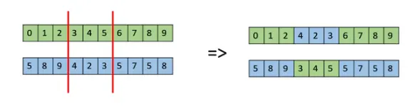
• CROSSOVER FUNCTION : This deals with mating of two individuals. Crossover done randomly by selecting the individuals by selection operator.

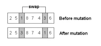
MUTATION FUNCTION : Inserting random genes in childrens to maintain the diversity among the population to avoid premature convergence.

Genetic Algorithm in MATLAB

In MATLAB GA can be utilized for finding the global minima for highly nonlinear problems. GAs can be applied to problems that are not well suited for standard optimization algorithms, including problems in which the objective function is discontinuous, modifiable, stochastic , or highly nonlinear.

Genetic Algorithm syntaxes used in MATLAB

• UNBOUNDED FUNCTION

x = ga(fun,nvars) finds a local unconstrained minimum, x, to the objective function, fun. nvars is the dimension (number of design variables) of fun.

• BOUNDED FUNCTION

x = ga(fun,nvars,A,b,Aeq,beq,lb,ub) defines a set of lower and upper bounds on the design variables, x, so that a solution is found in the range lb ≤ x ≤ ub. (Set Aeq=[] and beq=[] if no linear equalities exist.)

• BOUNDED INPUTS WITH POPULATION SIZE

x = ga(fun,nvars,A,b,Aeq,beq,lb,ub,nonlcon,options) minimizes with the default optimization parameters replaced by values in options. (Set nonlcon=[] if no nonlinear constraints exist.) Create options using optimoptions.

Terms used in the above syntaxes.

fun -functions

nvars - number of variables

A -linear inequality constraints

B -linear inequality constraints

Aeq -linear equality constraints

Beq -linear equality constraints

lb -ulowerbounds

ub -upper bounds

nonlcon -non linear constraints

For explaining the concept of genetic algorithm the formation of stalagmite is taken and the stalagmite function which represents the stalagmite growth is optimized by using the genetic algorithm function in matlab

Stalagmite

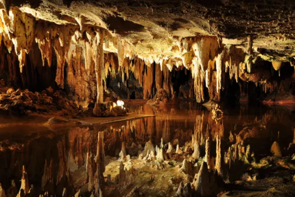
Stalagmite is an elongated form of various minerals deposited from solution by slowly dripping water. A stalactite hangs like ice hangs from the caves. A stalagmite appears like an inverted stalactite rising from the floors of caves.

Stalagmite Function

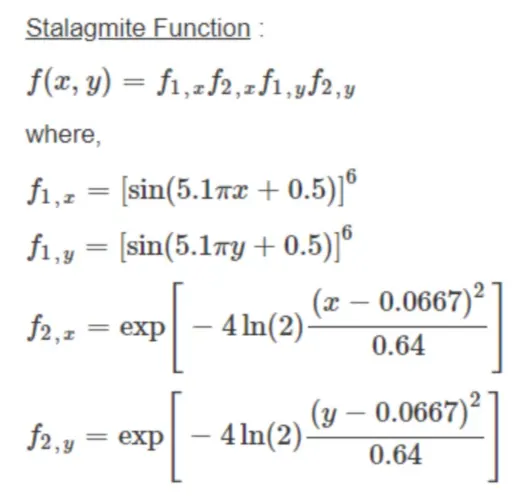
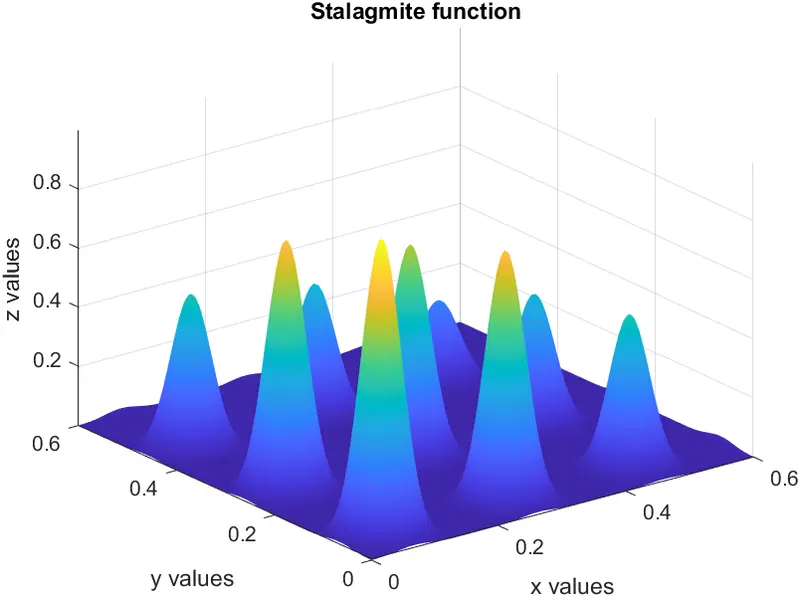
This function represents the stalagmite formation and its shape mathematically. Using this function, we will be able to plot the stalagmite formation. This mathematical stalagmite function is shown below.

Procedure.

Step 1

• Variables x and y are created using the linspace command. This will act as the search spaces and also using the meshgrid command inputs for the custom stalagmite function are created.

Step 2

• The custom stalagmite function is created on the basis of the above shown stalagmite mathematical equations.

Step 3

• Using the custom stalagmite function, ‘f’ is obtained.

Step 4

• Iterations are performed using a for loop.

Step 5

• The output is stored in the variable ‘fopt’.

Step 6

• UNBOUNDED FUNCTION, BOUNDED FUNCTION and BOUNDED INPUTS WITH POPULATION SIZE genetic algorithm syntaxes are executed under different study for optimization.

Step 7

• The computational time is noted using the TIC / TOC commands.

Step 8

• Using the outputs obtained, different plots are made.

Code

Stalagmite custom function

%Stalagmite function
function [y] = stalagmite_fn(input_vector)

x = input_vector(1);
y = input_vector(2);

f1 = (sin(5.1*pi*x + 0.5)).^6;
f2 = (sin(5.1*pi*y + 0.5)).^6;
f3 = exp(-4*log(2)*((x-0.0667)^2/0.64));
f4 = exp(-4*log(2)*((y-0.0667)^2/0.64));

y = -(f1*f2*f3*f4);
end

GENETIC ALGORITHM

%GENETIC ALGORITHM

clear all
close all 
clc

%Search Space
x = linspace(0,0.6,150);
y = linspace(0,0.6,150);

%2D array 

[xx yy] = meshgrid(x,y);

% Z element generation using the stalagmite function

for i = 1:length(xx)
    for j=1:length(yy)
        input_vector(1)= xx(i,j);
        input_vector(2)= yy(i,j);
        
       f(i,j) = stalagmite_fn(input_vector);
    end
end

%Plotting
figure(1)
surfc(xx,yy,-f)
title('Stalagmite function')
xlabel ('x values')
ylabel ('y values')
zlabel ('z values')
shading interp

% Optimized results using genetic algorithm

[output, fn_val] = ga(@stalagmite_fn,2);


%Displaying the output from the function as a table
Function_value = fn_val;
SF_Result = output;

Stalagmite_fn = table(output,Function_value)

%Number of iterations
num_case = 50;


%Study 1 : Unbounded Inputs

tic

for i = 1:num_case
    [input, fopt(i)] = ga(@stalagmite_fn,2);
    x_opt(i) = input(1);
    y_opt(i) = input(2);
end

%Computational time
case1_time = toc

%Plotting
figure(2)
subplot(2,1,1)
surfc(xx,yy,-f)
xlabel ('x values')
ylabel ('y values')
zlabel ('z values')
title('Study 1 : Unbounded Inputs')
shading interp

hold on

plot3(x_opt,y_opt,-fopt,'marker','o','markersize',5,'markerfacecolor','r')
subplot(2,1,2)
plot(-fopt)
xlabel('Cases')
ylabel('Max Function')




%Study 2 : Bounded inputs

tic

for i = 1:num_case
    [input, fopt(i)] = ga(@stalagmite_fn,2,[],[],[],[],[0;0],[0.6;0.6]);
    x_opt(i) = input(1);
    y_opt(i) = input(2);
end

%Computational time
case2_time = toc

%Plotting
figure(3)
subplot(2,1,1)
surfc(xx,yy,-f)
xlabel ('x values')
ylabel ('y values')
zlabel ('z values')
title('Study 2 : Bounded Inputs')
shading interp

hold on

plot3(x_opt,y_opt,-fopt,'marker','o','markersize',5,'markerfacecolor','r')
subplot(2,1,2)
plot(-fopt)
xlabel('Cases')
ylabel('Max Function')




%Study 3 : Bounded inputs with population size


options =optimoptions('ga');
options =optimoptions(options, 'PopulationSize',350);

tic

for i = 1:num_case
    [input, fopt(i)] = ga(@stalagmite_fn,2,[],[],[],[],[0;0],[0.6;0.6],[],[],options);
    x_opt(i) = input(1);
    y_opt(i) = input(2);
end

%Computational time
case3_time = toc

%Plotting
figure(4)
subplot(2,1,1)
surfc(xx,yy,-f)
xlabel ('x values')
ylabel ('y values')
zlabel ('z values')
title('Study 3 : Bounded Inputs with population size')
shading interp

hold on

plot3(x_opt,y_opt,-fopt,'marker','o','markersize',5,'markerfacecolor','r')
subplot(2,1,2)
plot(-fopt)
xlabel('Cases')
ylabel('Max Function')

%Displaying the funtion results and processing time of studies in a table
Stalagmite_fn = table(SF_Result,Function_value,case1_time,case2_time,case3_time)

Output

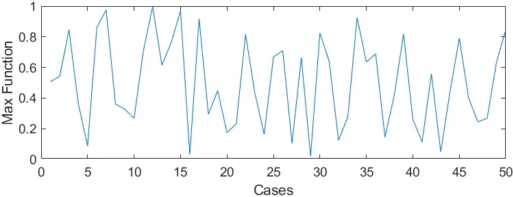
Study 1 : Unbounded inputs

x = ga(fun,nvars)

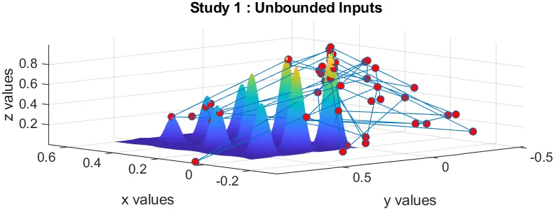
In this study the GA takes the values randomly so new output is generated every time the code is executed. That we can observe from this output, the values are all over the graph as the number of iteration took place is way too high.

Study 2 : Bounded inputs

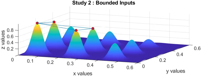
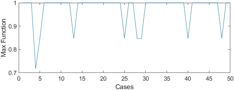
x = ga(fun,nvars,A,b,Aeq,beq,lb,ub)

In this study ,boundary values are provided into the GA so the output will be little more reliable and repeated comparing the previous scenario

Study 3 : Bounded inputs with population size

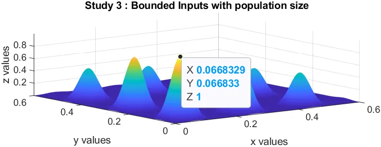
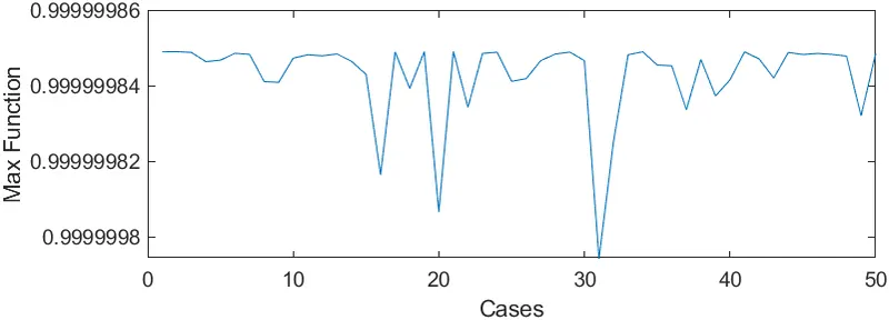
x = ga(fun,nvars,A,b,Aeq,beq,lb,ub,nonlcon,options)

In this study we specified the boundary conditions a little more by providing upper and lower boundary conditions and the population size. As a result we obtained a more specific and accurate global maxima.

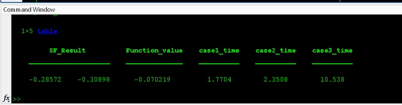
From this output we can observe that , as we provide more conditions to GA , the computational time increases.

Conclusions and observations

• The global maxima of the stalagmite function is found out in the last study
• The concepts of the genetic algorithms are explored.
• Different plots have been made using the datas that have been collected.
• From three studies it is observed that as we provide more conditions to the GA , the computational time also increases.

References :

Stalactite and stalagmite | Mineral formation | Britannica

Genetic Algorithms - GeeksforGeeks

Genetic Algorithm - MATLAB & Simulink (mathworks.com)

Find minimum of function using genetic algorithm - MATLAB ga - MathWorks India