Week 4.1 - Genetic Algorithm

Optimization of Stalagmite function and determination of global maxima by using Genetic algorithm

Stalagmites are geological mineral-rock formations that are commonly found in caves. These structures that rise pointing upward from the floor of the cave. Similar pointed structures can be found hanging from the roof of caves and are called stalactites. A stalagmite function is so called because its graphical surface representation resembles that of stalagmites rising from a plane (usually x-y plane). This function produces a number of local maximum and local minimum values and one global maxima and minima.

Mathematical equation of a stalagmite function is

`f(x,y)=[sin⁡(5.1πx+0.5) ]^6×[sin⁡(5.1πy+0.5) ]^6×e^[-4*ln⁡(2)*(x-0.0667)^2/0.064] ×e^[-4*ln⁡(2)*(y-0.0667)^2/0.064]`

Genetic Algorithm in programming is similar to its biological definition in that it repeatedly modifies a population (of solutions, in case of programming). At each step, the genetic algorithm randomly selects individuals from the current population and uses them as parents to produce the children for the next generation. Over successive generations, the population "evolves" toward an optimal solution. This process is done in 3 steps:

• Selection: It selects a number of individuals (set of solutions) based on some defined parameter (called fitness value). These individuals are called parents and they contribute to populate the next generation (iteration).
• Crossover: It combines or mutates parents (solutions) from a previous generation to form the next generation of offspring (again, solutions). The new offspring carries a random amount of genetic material from the previous generations.
• Mutation: Some offspring may change its genetic composition to form a new individual offspring.

In programming, the algorithm returns the Global Minimum value. It first creates a solution set at random, but confined within the limits of a fitness value through Selection process. It may then make random changes to the solutions to create the next solution set through Mutation method or combine vector quantities of two parent solutions to create the next solution set through Crossover method. Combination of the above steps keeps on creating new solution sets, each better than the last, until a limiting factor of the iteration (limit of fitness value, time limit etc) is reached.

In MATLAB, this algorithm is a solver called ‘ga’, which requires at least 2 input arguments; a fitness function (stalagmite function in this case) and the number of variables in the problem (x & y, so 2 variables). The first two output arguments returned by ga are x, the best point found, and fval, the function value at the best point.

Thus the basic syntax of ga solver is

[x,fval]=ga(fitness_function,number_of_variables)

Further, extra parameters can be passed to make the solver more efficient.

For the following line of code, ga solver returns a local minimum ‘x’ to the fitness function.

[x,fval]=ga(fitness_function,number_of_variables,a,b,a_eq,b_eq,lb,ub, nonlcon,intcon,options) 

Here, a and b are linear inequalities such that a*x ≤ b. Similarly, a_ep and b_eq are linear equalities such that a_eq*x = b_eq. These parameters are not used in this program.

lb and ub defines a set of lower and upper bounds on the output x so that a solution is found in the range lb≤x≤ub.

nonlcon and intcon are non-linear constraints and Integer constraints respectively, and are not used in this program.

options parameter creates options for optimization. It is used in this program in Study 3 to increase the number of iterations.

Since ga solver starts with a random initial population created using random number generators and since every time a random number is generated, the state of the random number generators changes, the results obtained each time the program is run changes when the mentioned parameters are not defined. This can be solved by resetting the random number generator stream as shown

state_of_stream=rng;

and adding the following line of code before using the ga solver.

rng(state_of_stream);

Code for stalagmite function:

%Stalagmite fuction
function[f]=stalagmite(input_vector)
x=input_vector(1);
y=input_vector(2);

f1_x=(sin((5.1*pi*x)+0.5))^6;
f1_y=(sin((5.1*pi*y)+0.5))^6;
f2_x=exp(-4*log(2)*((x-0.0667)^2)/0.64);
f2_y=exp(-4*log(2)*((y-0.0667)^2)/0.64);

f=-(f1_x*f1_y*f2_x*f2_y);
end

Code for genetic algorithm to solve stalagmite function for global maxima:

clear all
close all
clc

%Define search space
x=linspace(0,0.6,150);
y=linspace(0,0.6,150);
N=100;      %number of iterations

%Creating a 2D mesh
[xx yy]=meshgrid(x,y);

%Evaluating the stalagmite function
for i=1:length(xx)
    for j=1:length(yy)
        input_vector(1)=xx(i,j);
        input_vector(2)=yy(i,j);
        f(i,j)=stalagmite(input_vector);
    end
end

%Study 1- Statistical behaviour with unbounded inputs
tic     %stopwatch timer to record study run time
for i=1:N
    [output1,f_opt1(i)]=ga(@stalagmite,2);    %ga solver returns output and optimal                      %function value for each iteration
    x_opt1(i)=output1(1);      %x_opt1 stores optimal values for each iteration
    y_opt1(i)=output1(2);      %y_opt1 stores optimal values for each iteration
end
study_time_1=toc        %stores run time

%plotting
figure(1)

subplot(2,1,1)  
hold on
surfc(xx,yy,-f)     %3D surface plot
grid on 
shading interp
xlabel('x axis')
ylabel('y axis')
plot3(x_opt1,y_opt1,-f_opt1,'marker','diamond','MarkerSize',6,'MarkerFaceColor','Red')  %3 axis plot over surface plot
title('Statistical behaviour of ga solver (unbounded inputs)')

subplot(2,1,2)  %subplot shows optimal values in 2D
plot(-f_opt1)
xlabel('No. of iterations')
ylabel('Maximum function value')


%Study 2- Statistical behaviour with bounded inputs
tic
for i=1:N
    [output2,f_opt2(i)]=ga(@stalagmite,2,[],[],[],[],[0;0],[1;1],[],[]);  %'[]' are empty %because no parameters are defined  
    x_opt2(i)=output2(1);  
    y_opt2(i)=output2(2);
end
study_time_2=toc

%plotting
figure(2)

subplot(2,1,1)  
hold on
surfc(xx,yy,-f)     
grid on 
shading interp
xlabel('x axis')
ylabel('y axis')
plot3(x_opt2,y_opt2,-f_opt2,'marker','diamond','MarkerSize',6,'MarkerFaceColor','Red')  %3 axis plot over surface plot
title('Statistical behaviour of ga solver (bounded inputs)')

subplot(2,1,2)  
plot(-f_opt2)
xlabel('No. of iterations')
ylabel('Maximum function value')

%Study 3- Statistical behaviour with increased iterations (100 to 600)
options=optimoptions('ga');
options=optimoptions(options,"PopulationSize",600);

tic
for i=1:N
    [output3,f_opt3(i)]=ga(@stalagmite,2,[],[],[],[],[0;0],[1;1],[],[],options);    
    x_opt3(i)=output3(1);  
    y_opt3(i)=output3(2);
end
study_time_3=toc

%plotting
figure(3)

subplot(2,1,1)  
hold on
surfc(xx,yy,-f)     
grid on 
shading interp
xlabel('x axis')
ylabel('y axis')
plot3(x_opt3,y_opt3,-f_opt3,'marker','diamond','MarkerSize',6,'MarkerFaceColor','Red')  %3 axis plot over surface plot
title('Statistical behaviour of ga solver (increased iterations)')

subplot(2,1,2)  
plot(-f_opt3)
xlabel('No. of iterations')
ylabel('Maximum function value')

%end of code

Explanation:

The stalagmite function is defined as shown in the code and formula mentioned above. A negative sign was added to the output of stalagmite function so that the ga solver finds the maximum values instead of minimum values (which it is designed to do).

In the program for ga solver, initially, arrays 'x' and 'y' that store random values are created. The number of iterations (generations) that the ga would initally perform is defined by a variable 'N'. Using meshgrid function, the coressponding 2D mesh is created. To evaluate the stalagmite function, a nested for loop is used. This operation assign values to an array called 'input_vector', which is an input for the stalagmite function defined above.

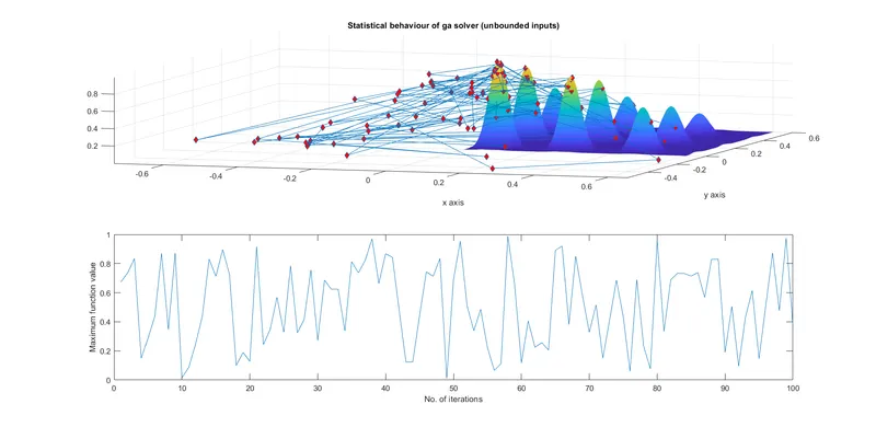
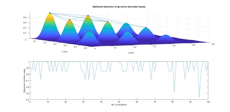
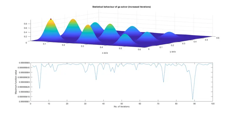
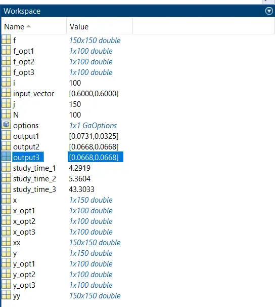
For the first study, the ga solver is defined within a for loop that runs till 'N' times. The ga solver is defined without any additional parameters other than the two output arguments. 'tic' and 'toc' stopwatch commands are used to get an idea about the program run time. Then the plots are made; first plot is the 3D surface plot, next the output values (denoted by red diamonds) are plotted and connected to each other. second plot is a 2D plot which shows optimal function values.

For the second study, bound parameters are added to the ga solver syntax.

For the third study, options parameter is added. The definition for options function is also added such that the number of iterations (PopulationSize) is increased to 600, which ultimately finds the perfect Global Maxima.

Results:

Study 1- Statistical behaviour with unbounded inputs: It is observed that the ga solver creates an unique optimum value with every iteration.

Study 2- Statistical behaviour with bounded inputs: When the solver inputs are bounded, there is a greater convergence of x and y values.

Study 3- Statistical behaviour with increased iterations (100 to 600): Once number of iterations was increased to 600, all x and y values convereged, thus returning the Global Maxima point at x=0.0668 and y=0.0668.

Values from workspace:

Referred links:

https://in.mathworks.com/discovery/genetic-algorithm.html

https://in.mathworks.com/help/gads/options-in-genetic-algorithm.html

https://www.youtube.com/watch?v=mwaDPAn0e7s&ab_channel=SolvingOptimizationProblems

https://in.mathworks.com/help/gads/ga.html#d123e44433

https://in.mathworks.com/help/optim/ug/optim.problemdef.optimizationproblem.optimoptions.html