Challenge

Project 1 - Parsing NASA thermodynamic data

AAneesh Kashyap7 Feb 2022

Parsing a thermodynamic data file and calculation of thermodynamic properties

In programming, data parsing is the process in which a string of data is converted from one format to another for various uses, for e.g. perform complex calculations, represent equations etc.

NASA’s thermodynamic data file contains data for chemical species (elements, compounds, isotopes etc). These data typically provide the thermodynamic properties (enthalpy, entropy, and specific heat) of a species as a function of temperature. The data obtained from the file can be used for complex calculations, simulation of complex reactions etc. According to the given data file, the data is in a format called CHEMKIN-II and data for each species can be represented by NASA polynomials as

H/RT = a1 + a2 T /2 + a3 T² /3 + a4 T³ /4 + a5 T⁴ /5 + a6/T

S/R = a1 lnT + a2 T + a3 T² /2 + a4 T³ /3 + a5 T⁴ /4 + a7

Cp/R = a1 + a2 T + a3 T² + a4 T³ + a5 T⁴

where Cp= Specific Heat: Amount of heat required per unit mass to raise temperature by 273 K

R= Universal Gas constant (8.314)

T= Temperature

H= Enthalpy: Sum of Internal energy of a system plus the product of pressure & volume

S= Entropy: Thermal energy of a system per unit temperature

and a1, a2, a3, a4, a5, a6, and a7 are the numerical coefficients supplied in NASA thermodynamic files. The first 7 numbers starting on the second line of each species entry (five of the second line and the first two of the third line) are the seven coefficients (a1 through a7, respectively) for the high-temperature range (above 1000 K, the upper boundary is specified on the first line of the species entry). The following seven numbers are the coefficients (a1 through a7, respectively) for the low-temperature range (below 1000 K, the lower boundary is specified on the first line of the species entry).

Explanation:

First step is to figure out how to read, identify and store the data from the file. By using commands fopen, the given file ‘THERMO.dat’ is opened and assigned to a variable ‘file_1’. Next, the program starts to read line by line by using fgetl command.

The Global temperature data is then read from the header information. This is done by splitting the line using strsplit command with ‘ ‘ (space) as parameter. The three temperature values obtained are stored to a variable each, by using str2num command, which converts string data to numerical data. Next, an array ‘T’ is defined using linspace command which stores 1000 global temperature values ranging from low temperature vale to high temperature value. These values of T will be used during plotting.

Next, the comment lines are skipped by using a for loop and fgetl command to read each line.

Before entering the main for loop, value of Universal Gas Constant R is defined.

To read the main data (names of species, local temperature ranges and coefficients), of which each of the 53 species present take up 4 lines each, a for loop which runs from 1 to 53 is defined. In each iteration of the loop, the program will read 4 lines.

The first line consists of the species name and local temperature ranges. Species name is read by using a strsplit command with ‘ ‘ (space) as parameter, and assigning the 1^st element of the cell array as ‘species’ variable.

To read the Local temperature ranges, which is unique for each species, it is found that in the CHEMKIN-II format temperatures are present as ‘low temp, high temp, medium temp’, each at the same position from the end of line (counting from right). These temperature data starts after the alphanumeric string ‘G’ or ‘1G’. It is found that the species either have ‘G’ followed by 3 spaces, at which the low temperature value starts, or ‘1G’ followed by 3 spaces, at which the low temperature value starts. Following this logic, program finds ‘G ’ (G followed by ‘ ‘(space)) and then finds the position of the local temperature ranges. The temperature ranges thus obtained are used to define an array ‘T_local’ is defined using linspace command which stores 1000 values ranging from low temperature value to high temperature value. These values of T_local will be used to calculate the values of H, S and Cp in the function ‘therm_props’

Then the program reads next line, denoted as ‘line2’. Here, the coefficients have to be extracted; ‘line2’ contains 5 coefficients (high temperature), next line ‘line3’ contains the next 5, of which 3 are lower temperature coefficients. Next line ‘line4’ contains the last 4 lower temperature coefficients. Extracting each is done by finding ‘E’ (which is present for all coefficients) and then reading from that position till 3 units after ‘E’. This is repeated till a1 through a14 are obtained and stored.

Next, ‘therm_props’ function is called. This function takes all the extracted coefficients, ‘T_local’, R and Local Medium temperature and calculates and returns H, S and Cp for each species.

Then, function for molecular weight is called, which compares the name of species to a user defined array ‘elements’ which contains the basic elements that makes up different species in the file. If the comparison holds true, it assigns the molecular weight from another user defined array ‘atom_weight’ containing atomic weights of respective elements in the ‘elements’ array. The function also checks for number of elements in each species and if there is more than 1 element present, the for loop runs again till total molecular weight is calculated.

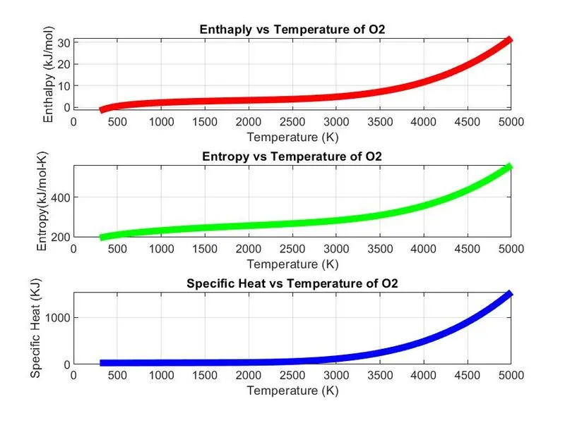
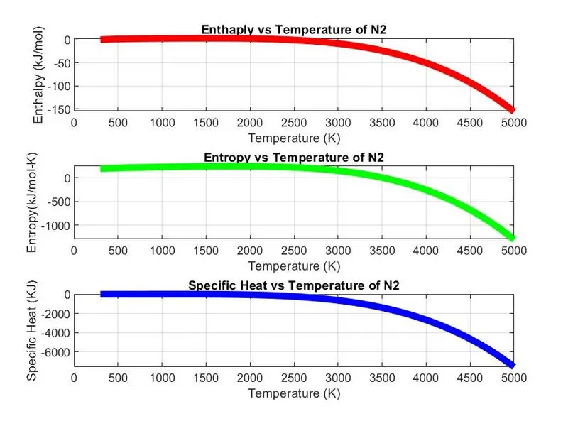
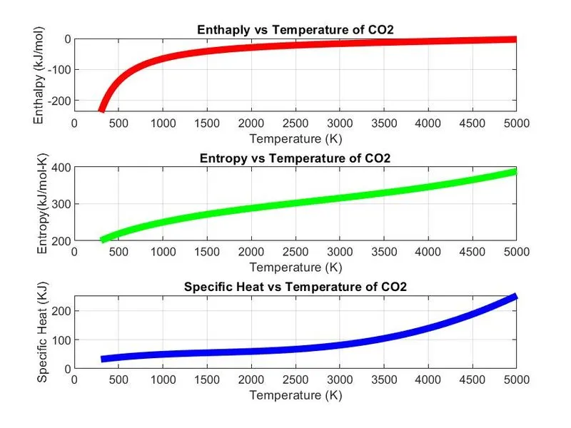
Plotting is done next. To save each plot in an unique folder for each species, a new directory is make using mkdir command. Plotting for Enthalpy ‘H’, Entropy ‘S’ and Specific Heat ‘Cp’ against Global temperature ‘T’ is done. cd command changes the directory to the newly made directory for plots to be saved in. saveas command is used to save the figure containing all 3 subplots.

Main Program Code:

%Main Program
clc
close all
clear all

%Opening given THERMO.dat file
file_1=fopen("THERMO.dat",'r');      %File opened and ready to be read
f=fgetl(file_1);

%Reading header info- Temperature data
Temp_header_line=fgetl(file_1);
temp=strsplit(Temp_header_line,' ');  
Global_temp_low=str2num(temp{2});   %Converting string data to numerical data
Global_temp_med=str2num(temp{3});
Global_temp_high=str2num(temp{4});
T=linspace(Global_temp_low,Global_temp_high,1000);   %Temp range defined

%Skipping 3 comment lines 
for i=1:3
    f=fgetl(file_1);
end

%Defining Universal Gas Constant R
R=8.314;


%Reading names and coefficients of 53 species
for j=1:53
    line1=fgetl(file_1);        %reading line 1
    x=strsplit(line1,' ');      %x becomes a cell array
    species=(x{1});             %'species' stores names of species

    %Reading Local temperature range
    g=findstr(line1,'G ');
    local_temp_low=line1(g+3:g+9);  %starting position of temp data to end
    local_temp_low=str2num(local_temp_low);   %Converting string data to numerical data
    local_temp_high=line1(g+12:g+19);
    local_temp_high=str2num(local_temp_high);
    local_temp_med=line1(g+22:g+29);
    local_temp_med=str2num(local_temp_med);
    T_local=linspace(local_temp_low,local_temp_high,1000);   %Temp range defined
    
    line2=fgetl(file_1);        %reading next line (line 2)
    e2=findstr(line2,'E');      %finding E among coefficients data
                                %'e2' denotes E character in line 2
    %Extracting coefficients a1 through a7 (higher temp coeff)
    a1=line2(1:e2(1)+3);
    a1=str2num(a1);             %Coefficient a1
    a2=line2(e2(1)+4:e2(2)+3);
    a2=str2num(a2);             %Coefficient a2
    a3=line2(e2(2)+4:e2(3)+3);
    a3=str2num(a3);             %Coefficient a3
    a4=line2(e2(3)+4:e2(4)+3);
    a4=str2num(a4);             %Coefficient a4
    a5=line2(e2(4)+4:e2(5)+3);
    a5=str2num(a5);             %Coefficient a5
    
    line3=fgetl(file_1);        %reading next line (line 3)
    e3=findstr(line3,'E');      %finding E among coefficients data
                                %'e3' denotes E character in line 3
    a6=line3(1:e3(1)+3);
    a6=str2num(a6);             %Coefficient a6
    a7=line3(e3(1)+4:e3(2)+3);
    a7=str2num(a7);             %Coefficient a7

    %Extracting coefficients a8 through a14 (lower temp coeff)
    a8=line3(e3(2)+4:e3(3)+3);
    a8=str2num(a8);             %Coefficient a8
    a9=line3(e3(3)+4:e3(4)+3);
    a9=str2num(a9);             %Coefficient a9
    a10=line3(e3(4)+4:e3(5)+3);
    a10=str2num(a10);           %Coefficient a10

    line4=fgetl(file_1);        %reading next line (line 4)
    e4=findstr(line4,'E');      %finding E among coefficients data
                                %'e4' denotes E character in line 4
    a11=line4(1:e4(1)+3);
    a11=str2num(a11);           %Coefficient a11
    a12=line4(e4(1)+4:e4(2)+3);
    a12=str2num(a12);           %Coefficient a12
    a13=line4(e4(2)+4:e4(3)+3);
    a13=str2num(a13);           %Coefficient a13
    a14=line4(e4(3)+4:e4(4)+3);
    a14=str2num(a14);           %Coefficient a14
    
    %Calling function 'therm_props' 
    % and storing calculated vales of enthalpy, entropy and specific heat
    [H,S,Cp]= therm_props(a1,a2,a3,a4,a5,a6,a7,a8,a9,a10,a11,a12,a13,a14,T_local,R,local_temp_med);
    
    %Calling function 'mol_weight' to get Molecular weights of species
    mol_weight=molecular_weight(species);
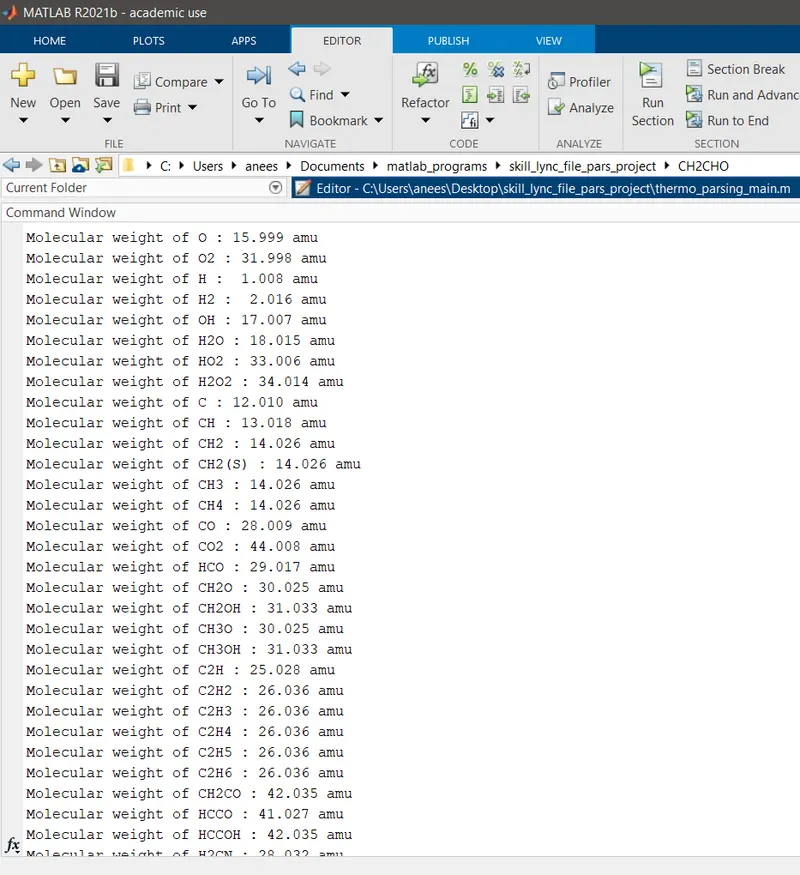
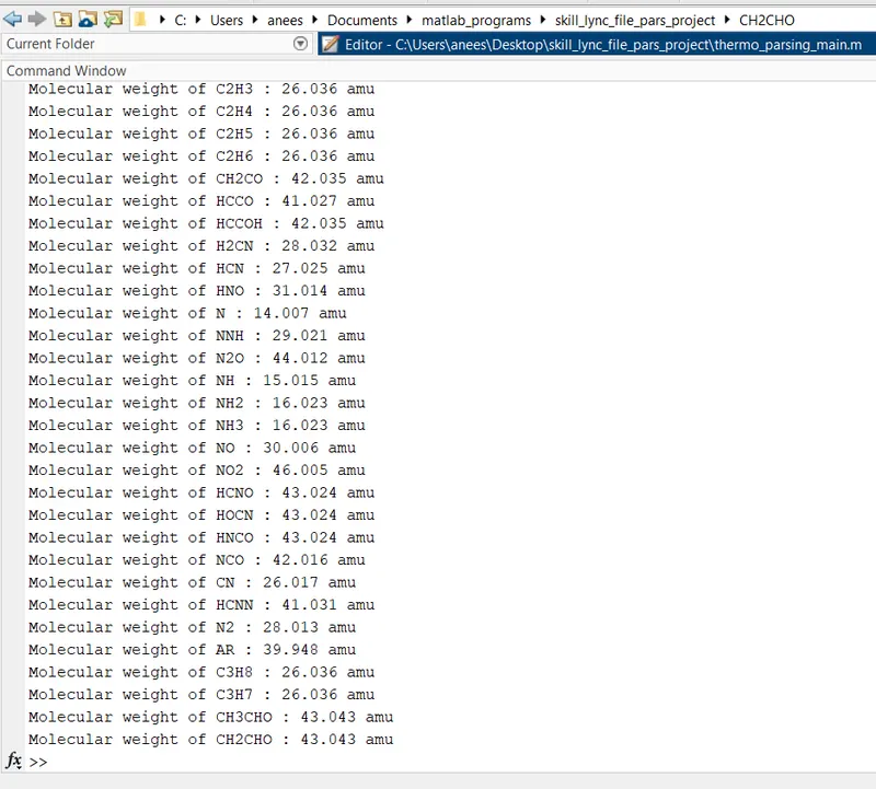
    fprintf('Molecular weight of %s : %6.3f amu \n',species,mol_weight);

    %Saving to separate folders
    %Making new directory to store plots
    mkdir(['C:\Users\anees\Documents\matlab_programs\skill_lync_file_pars_project\',species]);

    %Plots
    %H vs T
    figure(1)
    subplot(3,1,1)
    plot(T,H,'LineWidth',5,'Color','r');
    xlabel('Temperature (K)')
    ylabel('Enthalpy (kJ/mol)')
    title(sprintf('Enthaply vs Temperature of %s',species));
    grid on
    %S vs T
    figure(1)
    subplot(3,1,2)
    plot(T,S,'LineWidth',5,'Color','g');
    xlabel('Temperature (K)')
    ylabel('Entropy(kJ/mol-K)')
    title(sprintf('Entropy vs Temperature of %s',species));
    grid on
    %Cp vs T
    figure(1)
    subplot(3,1,3)
    plot(T,Cp,'LineWidth',5,'Color','b');
    xlabel('Temperature (K)')
    ylabel('Specific Heat (KJ)')
    title(sprintf('Specific Heat vs Temperature of %s',species));
    grid on
    
    %saving plots in the directory
    cd(['C:\Users\anees\Documents\matlab_programs\skill_lync_file_pars_project\',species]);
    saveas(figure(1),'Thermodynamic properties.jpg');
end

Function Codes:

%Function to calculate Enthalpy H, Entropy S, Specific Heat Cp
function [H,S,Cp]= therm_props(a1,a2,a3,a4,a5,a6,a7,a8,a9,a10,a11,a12,a13,a14,T_local,R,local_temp_med)

%Comparing Temp range with Global temp 1000 K
    if T_local>=local_temp_med
        %Formula for Enthalpy H
        H=(a1+((a2*T_local)/2)+((a3*T_local.^2)/3)+((a4*T_local.^3)/4)+((a5*T_local.^4)/5)+(a6./T_local));
        %Formula for Entropy S
        S=(a1.*log(T_local)+(a2*T_local)+((a3*T_local.^2)/2)+((a4*T_local.^3)/3)+((a5*T_local.^4)/4)+a7)*R;
        %Formula for Specific Heat Cp
        Cp=(a1+(a2*T_local)+(a3*T_local.^2)+(a4*T_local.^3)+(a5*T_local.^4))*R;
    else
        H=(a8+((a9*T_local)/2)+((a10*T_local.^2)/3)+((a11*T_local.^3)/4)+((a12*T_local.^4)/5)+(a13./T_local));
        S=(a8.*log(T_local)+(a9*T_local)+((a10*T_local.^2)/2)+((a11*T_local.^3)/3)+((a12*T_local.^4)/4)+a14)*R;
        Cp=(a8+(a9*T_local)+(a10*T_local.^2)+(a11*T_local.^3)+(a12*T_local.^4))*R;
    end
end

%Function to calculate Molecular weights of species
function mol_weight=molecular_weight(species)
         %Creating an array to store names of each element 
         elements=['H','C','N','O','Ar'];
                  
         %Creating an array to store atomic weights of each element
         atom_weight=[1.0079 12.010 14.0067 15.999 39.948];

         mol_weight=0;  %Assigning a starting value 
         for x=1:length(species)
             for y=1:length(atom_weight)
                 if strcmpi(species(x),elements(y)) %comparing 
                     mol_weight=mol_weight+atom_weight(y);
                     cntr=y;    %counter
                 end
             end
             n=str2num(species(x));
             if n>1
                 mol_weight=mol_weight+atom_weight(cntr);
             end
         end
end

Results:

Molecular weights displayed in command window-

Folder containing plots-

Thermodynamic properties plots for

a. O2-

b. N2-

c. CO2-

Errors:

Some errors in syntax were faced, but fixed during a one-on-one session, of which unfortunately no screenshots were preserved. No other major errors were faced.

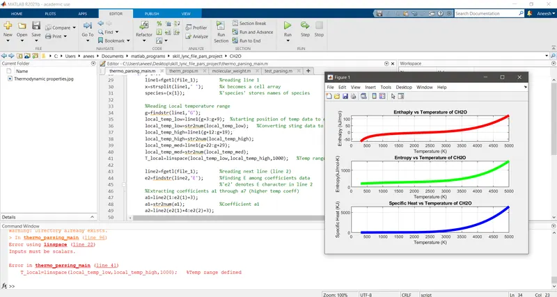
The following error 'Inputs must be in scalar' for linspace command is because the presence of '1G' while finding for the string ' G ' (space G space) was not accounted for.