Week 3 - Solving second order ODEs

Solving 2nd order ODE to visualize angular displacement and angular velocity curves of a simple pendulum and to animate its motion

A differential equation is a mathematical equation that contains at least one derivative term of a variable (say, x) as a function of another variable (say, y). An ordinary differential equation (ODE) is an equation that involves ordinary derivatives of a function. In engineering terms, a differential equation is a mathematical representation of a dynamic system (mechanical, electrical, hydraulic, etc.). It helps in understanding the dynamic behaviour of a system.

A 2^nd order ODE is one in which the derivative corresponding to the independent variable is raised to the power of 2.

A simple pendulum has a point mass ‘m’ (usually a ball) suspended from a point by a string or wire of length ‘l’ and negligible mass. When the mass is displaced to an angle θ w.r.t. the vertical and released, the pendulum starts to oscillate about its mean position in a periodic motion known as Simple Harmonic Motion (SHM). The basic theory of a simple pendulum applies to a vehicle’s suspension system, which comprises of a spring, damper and the weight of the vehicle considered as a point mass.

For a pendulum, if ‘m’ is the mass of the ball, ‘l’ is the length of the string, ‘b’ is the damping coefficient and ‘g’ represents the accleration due to gravity and the mass is displaced by an initial angle of θ, its motion is governed by the following equation:

`(d^2 θ)/(dt^2 )+b⁄m (dθ)/dt+g⁄l sin⁡θ=0`

To get the solution of this equation, let us consider

`θ=θ_1`

Taking derivatives on both sides,

`(dθ)/dt=(dθ_1)/dt=θ_2 (say)`

Taking derivatives on both sides again,

`(d^2 θ)/(dt^2 )=(d^2 θ_1)/(dt^2 )=(dθ_2)/dt`

Substituting `(dθ_2)/dt=(d^2 θ)/(dt^2 )`

`(dθ_2)/dt+(b⁄m) θ_2+(g⁄l) sin⁡θ_1=0`

`(dθ_2)/dt=-(b⁄m) θ_2-(g⁄l) sinθ_1`

Representing in matrix form,

`d/dt [(θ_1),(θ_2) ]=[(θ_2),(-b⁄m θ_2-g⁄l sin⁡θ_1) ]`, which gives the solution set.

Explanation:

The inputs are defined as given in the problem.

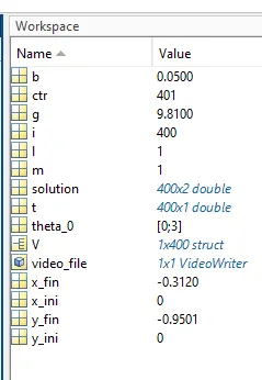
• Damping coefficient ‘b’= 0.05
• Acceleration due to gravity ‘g’=9.81 (in m/s^2)
• Length of string ‘l’= 1 (in m)
• Mass ‘m’= 1 (in kg)

Initial conditions are also provided. Thus, at time ‘t’=0,

• Angular displacement= 0
• Angular velocity= 3 (rad/sec)

The simulation has to be done for 20 seconds, therefore an array ‘theta_0’ is defined using linspace command. This array stores 400 time values from 0 to 20 seconds.

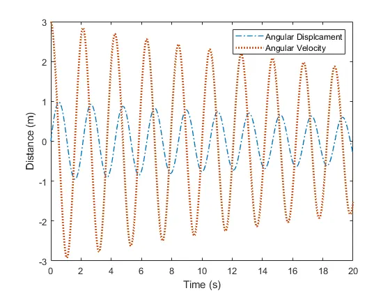
For solving the ODE, MATLAB solver ode45 is used. The results are stored in a 2 column matrix of 400 rows ‘solution’, which uses the ode45 solver and calls a user defined function ‘ode_func’. This function takes t, theta, b,g,l and m as inputs to calculate the solution set, as per the formulae explained above. The angular displacement and angular velocity were plotted from the obtained solution.

To animate the motion of pendulum, firstly, a for loop was used. The coordinates of initial and final postions were defined.

For initial position, (x,y)=(0,0).

For final position, (x,y)=(lsinθ,-lcosθ)

The plot commands were defined for the plane fromwhich the pendulum hangs, the string and the point mass.

Next, movie(V) command is used to stitch all the frames from array V to create a video file. The remaining commands are about specifing video file name (to be saved as .avi format), opening the video file, writing to it and closing.

Code:

%Solving 2nd order ODE to visualize angular displacement and 
%angular velocity curves of a simple pendulum and to animate its motion  
clear all
close all
clc

%Known inputs
b=0.05;         %Damping coefficient
m=1;            %Mass of ball in kg
l=1;            %Length of pendulum in m
g=9.81;         %Acceleration due to gravity in m/s^2

%Initial conditions at time t=0
theta_0=[0;3];  %theta_0=[angular displacement; angular velocity]

%Time array to define integration limits
t=linspace(0,20,400);

%Solving ODE
%Solution of ODE depends on time t and angle theta
[t,solution]=ode45(@(t,theta)ode_func(t,theta,b,g,l,m),t,theta_0);

%Plotting angular displacement and angular velocity
figure(1)
plot(t,solution(:,1),"LineStyle","-.","LineWidth", 1)   %Displacement curve
hold on
plot(t,solution(:,2),"LineStyle", ":", "LineWidth", 2)  %Velocity curve
xlabel('Time (s)')
ylabel('Distance (m)')
legend("Angular Displcament", "Angular Velocity", "Box","on")

%Animation
ctr=1;                              %Counter
for i=1:length(solution(:,1))   
    x_ini=0;                        %x-coordinate of initial position 
    y_ini=0;                        %y-coordinate of initial position
    x_fin=l*sin(solution(i,1));     %x-coordinate of final position 
    y_fin=-l*cos(solution(i,1));    %y-coordinate of final position 
    figure(2)
    %Plotting the plane from which pendulum hangs
    plot([-1 1],[0 0], "LineWidth",2,"Color",'b')   
    hold on
    %Plotting the string
    plot([x_ini x_fin],[y_ini y_fin], "LineWidth",2,"Color",'y')
    hold on
    %Plotting the ball
    plot(x_fin, y_fin, 'o', 'MarkerSize', 15, 'MarkerFaceColor', 'y', 'MarkerEdgeColor', 'r')
    axis([-1.5 1.5 -1.5 1])
    pause(0.01)
    hold off
    V(ctr)=getframe(gcf);   %V array stores frames of the plot
    ctr=ctr+1;              %counter incremented
end

movie(V)                    %movie command to generate video
video_file=VideoWriter('Pendulum_ode_solve.avi', 'Uncompressed AVI');
open(video_file);
writeVideo(video_file,V);
close(video_file);

Function code:

function [dtheta_dt]=ode_func(t,theta,b,g,l,m)
theta1=theta(1);
theta2=theta(2);
dtheta1_dt=theta2;
dtheta2_dt=-(b/m)*theta2-(g/l)*sin(theta1);
dtheta_dt=[dtheta1_dt;dtheta2_dt];
end

Values from workspace:

The plot obtained is as follows.

The animation was tried to be uploded to Youtube, but upon multiple tries, it showed 'Error 503' from both Chrome and Firefox browser.

Therefore a GDrive link to the animation is provided:

Animation of SHM motion for a simple pendulum

Errors:

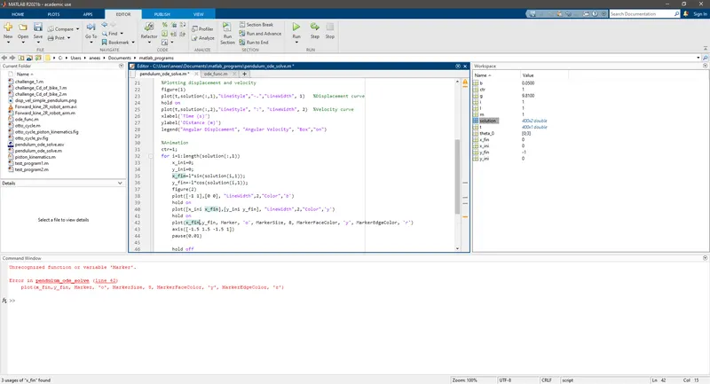
The following error was shown because of incorrect syntax while defining Marker size, Marker face color and marker edge color in line 42 (line 47 in the final code)