Project 2 - Rankine cycle Simulator
Simulation of Rankine cycle
The Rankine cycle is type of thermodynamic cycle of a constant pressure heat engine (steam engine) that converts part of heat into mechanical work. In this cycle, the heat is supplied externally to a closed loop, which usually uses water (in a liquid and vapour phase) as the working fluid. It is a modified form of Carnot cycle in which the Isothermal Compression is continued until the steam is condensed into water.
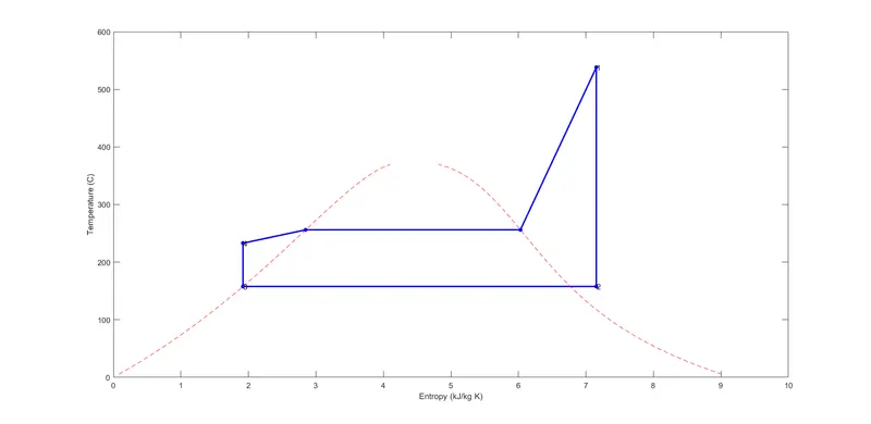
The following is a T-S diagram of an ideal Rankine cycle
The Rankine cycle operates in the following steps:
1-2 Isentropic Expansion- Here, water is in the form of superheated steam and it expands in the turbine, thus producing mechanical work. As work is being done on the turbine blades, the superheated steam turns into a mixture of vapour and liquid. Considering H1 and H2 as Enthalpies at states 1 and 2 respectively, work obtained at the turbine is expressed as-
WTurbine=H1-H2
2-3 Isobaric Heat Rejection- The saturated vapour-liquid mixture leaving the turbine is condensed to a complete liquid state at low pressure in a heat exchanger (condenser) using cooling water. Considering H2 and H3 as Enthalpies at states 2 and 3 respectively, heat rejected at the condenser is expressed as-
QRej=H2-H3
3-4 Isentropic Compression- Here, a feed pump is used to raise the pressure of the saturated water before entering the boiler. Considering H4 and H3 as Enthalpies at states 4 and 3 respectively, work done by the pump is expressed as-
WPump=H4-H3
4-1 Isobaric Heat Addition- High pressure liquid enters the boiler from the feed pump and is heated to the saturation temperature. Further addition of energy causes evaporation of the liquid until it is fully converted to saturated steam. Considering H1 and H4 as Enthalpies at states 1 and 4 respectively, heat added at the boiler is expressed as-
QAdd=H1-H4
The Net work output of a Rankine cycle is expressed as
Net Work Output= WTurbine-WPump
The Back work ratio is a way to describe the performance of the pump. It is expressed as
BWR= WPump/ WTurbine
The following is a MATLAB code for a simple ideal Rankine cycle, without reheating or regeneration.
%Simulation of Rankine cycle
clear all
close all
clc

%Processes
fprintf('1-2 Isentropic expansion (in turbine)\n')
fprintf('2-3 Isobaric heat rejection (in heat exchanger)\n')
fprintf('3-4 Isentropic compression (in pump)\n')
fprintf('4-1 Isobaric heat addition (in boiler)\n')

%Inputs
T1=input('Enter Turbine Inlet Temperature (C):');
P1=input('Enter Turbine Inlet Pressure (bar):');
P2=input('Enter Turbine Outlet Pressure (bar):');

%Calculation of State properties
%at state 1 (Superheated vapour)
h1_vapour=XSteam('hV_p',P1);
s1_vapour=XSteam('sV_p',P1);
cp1_liquid=XSteam('CpL_p',P1);
cp1_vapour=XSteam('CpV_p',P1);
t1_sat=XSteam('Tsat_p',P1);

%at state 2 (Saturated mixture)
h2_vapour=XSteam('hV_p',P2);
h2_liquid=XSteam('hL_p',P2);
s2_vapour=XSteam('sV_p',P2);
s2_liquid=XSteam('sL_p',P2);
cp2_vapour=XSteam('CpV_p',P2);
cp2_liquid=XSteam('CpL_p',P2);
t2_sat=XSteam('Tsat_p',P2);

%at state 3 (Saturated water)
P3=P2;
h3_liquid=XSteam('hL_p',P3);
s3_liquid=XSteam('sL_p',P3);
T3=t2_sat;

%at state 4 (Compressed liquid water)
P4=P1;
h4_liquid=XSteam('hL_p',P4);
s4_liquid=XSteam('sL_p',P4);

%Calculation of Process properties
%at state 1 (Superheated vapour)
H1=XSteam('h_pT',P1,T1);
S1=XSteam('s_pT',P1,T1);

%at state 2 (Saturated mixture)
S2=S1;
%Dryness fraction
X2=(S2-s2_liquid)/(s2_vapour-s2_liquid);
T2=t2_sat;
H2=h2_liquid+X2*(h2_vapour-h2_liquid);

%at state 3 (Saturated water)
S3=s3_liquid;
H3=h3_liquid;

%at state 4 (Compressed liquid water)
S4=S3;
H4=XSteam('h_ps',P4,S4);
CP4=XSteam('Cp_ps',P4,S4);
CV4=XSteam('Cv_ps',P4,S4);
gamma4=CP4/CV4;
T4=T3*((P4/P3)^((gamma4-1)/gamma4));

%for process 4-1,
T5=t1_sat;
S5=XSteam('sL_p',P1);
S6=s1_vapour;

%Net Work output and BWR calculation
w_turbine=H1-H2;
w_pump=H4-H3;
w_net=w_turbine-w_pump;
back_work_ratio=w_pump/w_turbine;

%Plots
%Saturation curves for T-S and H-S plots
vap_liq_line=linspace(0,T1,100);
for i=1:length(vap_liq_line)
    s_liquid(i)=XSteam('sL_T',vap_liq_line(i));
    s_vapour(i)=XSteam('sV_T',vap_liq_line(i));
    h_liquid(i)=XSteam('hL_T',vap_liq_line(i));
    h_vapour(i)=XSteam('hV_T',vap_liq_line(i));
end

figure(1)
plot([S1 S2 S3 S4 S5 S6 S1],[T1 T2 T3 T4 T5 T5 T1],'Color','b','LineWidth',2,'Marker','*','MarkerSize',5,'MarkerFaceColor','r')
text(S1,T1,'1','FontSize',10)
text(S2,T2,'2','FontSize',10)
text(S3,T3,'3','FontSize',10)
text(S4,T4,'4','FontSize',10)
hold on
plot(s_liquid,vap_liq_line,'Color','r','LineStyle','--')
plot(s_vapour,vap_liq_line,'Color','r','LineStyle','--')
axis([0 10 0 600])
xlabel('Entropy (kJ/kg K)')
ylabel('Temperature (C)')

figure(2)
plot([S1 S2 S3 S4 S1],[H1 H2 H3 H4 H1],'Color','b','LineWidth',2,'Marker','*','MarkerSize',5,'MarkerFaceColor','r')
text(S1,H1,'1','FontSize',10)
text(S2,H2,'2','FontSize',10)
text(S3,H3,'3','FontSize',10)
text(S4,H4,'4','FontSize',10)
hold on
plot(s_liquid,h_liquid,'Color','r','LineStyle','--')
plot(s_vapour,h_vapour,'Color','r','LineStyle','--')
axis([0 10 200 4000])
xlabel('Entropy (kJ/kg K)')
ylabel('Enthalpy (kJ/kg)')

%Outputs
fprintf('\nResults\n')
fprintf('At State point 1:\nP1=%5.3f (bar)\nT1=%5.3f (C)\nS1=%5.3f (kJ/kg K)\nH1=%5.3f (kJ/kg)\n\n',P1,T1,S1,H1)
fprintf('At State point 2:\nP2=%5.3f (bar)\nT2=%5.3f (C)\nS2=%5.3f (kJ/kg K)\nH2=%5.3f (kJ/kg)\n\n',P2,T2,S2,H2)
fprintf('At State point 3:\nP3=%5.3f (bar)\nT3=%5.3f (C)\nS3=%5.3f (kJ/kg K)\nH3=%5.3f (kJ/kg)\n\n',P3,T3,S3,H3)
fprintf('At State point 4:\nP4=%5.3f (bar)\nT4=%5.3f (C)\nS4=%5.3f (kJ/kg K)\nH4=%5.3f (kJ/kg)\n\n',P4,T4,S4,H4)
fprintf('Net Work Output=%5.3f (kJ/kg)\n',w_net)
fprintf('Back work ratio=%8.7f\n',back_work_ratio)
Explanation-
The program starts by clearing the workspace and command window. The 4 processes of the Rankine cycle are then displayed after which the program asks for the following inputs, as given in the question:
Turbine Inlet Temperature (C), Turbine Inlet Pressure (bar) & Turbine Outlet Pressure (bar).
Based on the inputs provided, the State properties are calculated first with the help of XSteam command. XSteam is a type of steam table which programs can easily access and return values such as Temperature, Pressure, Volume, Enthalpy, Entropy etc. for various conditions.
Similarly, Process properties are calculated. Next, net work done and back work ratio are calculated using the formulae mentioned above.
To plot the saturation curves, an array ‘vap_liq_line’ to store the temperature range was defined using linspace command, where initial temperature is 0 and maximum temperature is taken as input (T1). Next, a for loop is used to store values for enthalpy and entropy; for each iteration of the loop, the enthalpy and entropy values are obtained from XSteam table and stored.
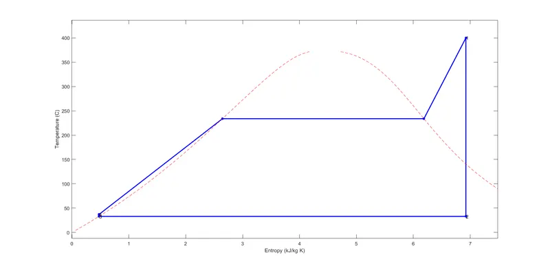
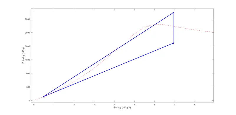
Next, the plots for T vs S and H vs S are made.
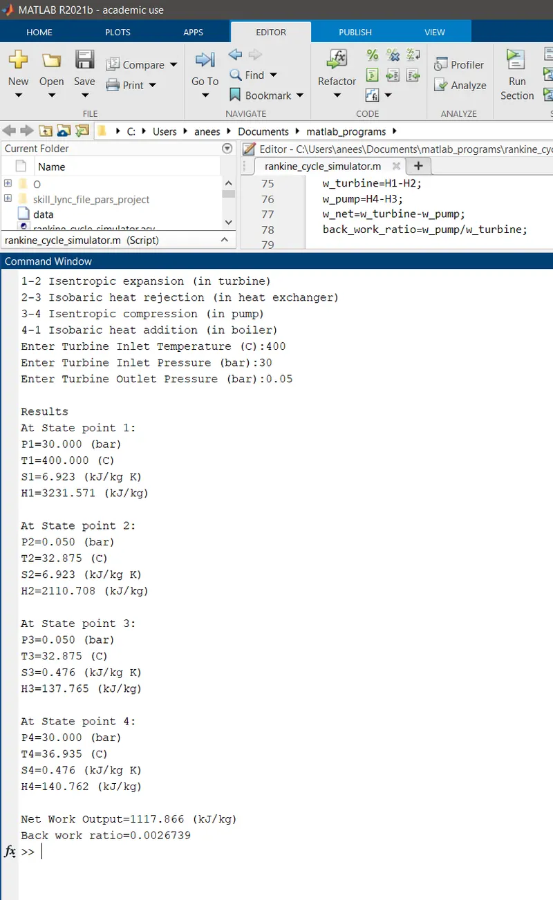
Lastly, the results were displayed in the command window.
Results-
a. T-S diagram:
b. H-S diagram:
c. Command window:
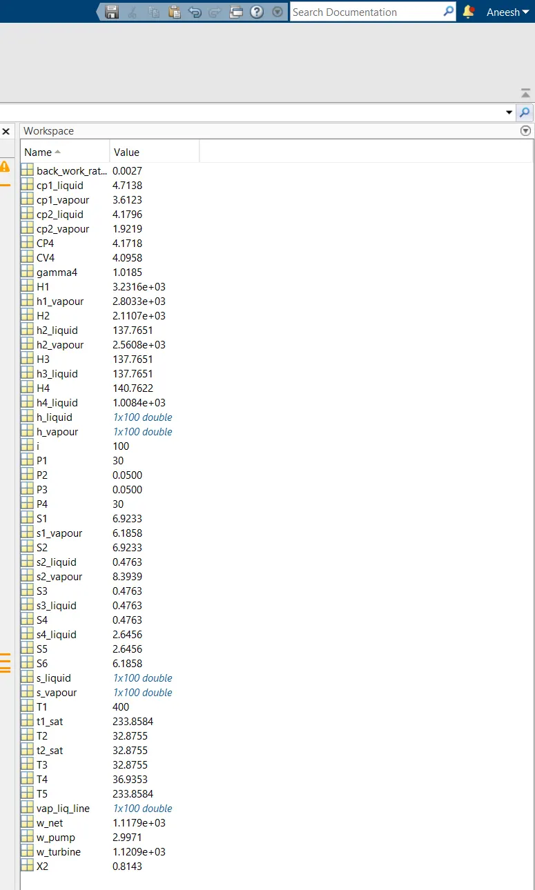
d. Workspace:
Errors:
Finding the value for T4 proved to be a slight issue. No major errors were faced.
Reference:
https://www.researchgate.net/figure/Back-work-ratio-all-cycles-and-working-fluids_tbl2_49128780
https://www.learnthermo.com/T1-tutorial/ch09/lesson-B/pg07.php
https://www.mechstudies.com/rankine-cycle-actual-diagrams-equations-formula/
https://www.theengineerspost.com/rankine-cycle/
https://old.amu.ac.in/emp/studym/99995366.pdf
https://ziegler.che.ufl.edu/Problem%20set%20solutions.pdf