Week 4.1 - Genetic Algorithm
Aim & Objective: To study about Genetic Algorithm, calculate the global maxima of stalagmite function using Genetic Algorithm in Matlab and plot graphs based on the studies.
Theory:
Concept of Genetic Algorithm:
A genetic algorithm (GA) is a method for solving both constrained and unconstrained optimization problems based on a natural selection process that mimics biological evolution. The algorithm repeatedly modifies a population of individual solutions. At each step, the genetic algorithm randomly selects individuals from the current population and uses them as parents to produce the children for the next generation. Over successive generations, the population "evolves" toward an optimal solution.
You can apply the genetic algorithm to solve problems that are not well suited for standard optimization algorithms, including problems in which the objective function is discontinuous, nondifferentiable, stochastic, or highly nonlinear.
The genetic algorithm differs from a classical, derivative-based, optimization algorithm in two main ways, as summarized in the following table.
|
Classical Algorithm |
Genetic Algorithm |
|
Generates a single point at each iteration. The sequence of points approaches an optimal solution. |
Generates a population of points at each iteration. The best point in the population approaches an optimal solution. |
|
Selects the next point in the sequence by a deterministic computation. |
Selects the next population by computation which uses random number generators. |
How the Genetic Algorithm Works:
The following outline summarizes how the genetic algorithm works:
- The algorithm begins by creating a random initial population.
- The algorithm then creates a sequence of new populations. At each step, the algorithm uses the individuals in the current generation to create the next population. To create the new population, the algorithm performs the following steps:
- Scores each member of the current population by computing its fitness value. These values are called the raw fitness scores.
- Scales the raw fitness scores to convert them into a more usable range of values. These scaled values are called expectation values.
- Selects members, called parents, based on their expectation.
- Some of the individuals in the current population that have lower fitness are chosen as elite. These elite individuals are passed to the next population.
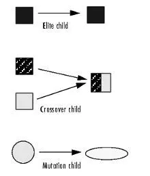
- Produces children from the parents. Children are produced either by making random changes to a single parent—mutation—or by combining the vector entries of a pair of parents—crossover. The following schematic diagram illustrates the three types of children.
- Replaces the current population with the children to form the next generation.
- The algorithm stops when one of the stopping criteria is met.
- The algorithm takes modified steps for linear and integer constraints.
- The algorithm is further modified for nonlinear constraints.
Syntax of ga Function:
x = ga(fun, nvars, A, b, Aeq, beq, lb ub,nonlcon,intcon,options);
defines a set of lower and upper bounds on the design variables, x, so that a solution is found in the range “lb <= x <= ub” and find minimum of the function. Where,
fun – function
nvars – number of variables
A – linear inequality constraints
b – linear inequality constraints
Aeq – linear inequality constraints
beq – linear inequality constraints
lb – lower bound
ub – upper bound
nonlcon - Non linear Inequalities
intcon - Integer constrained
options - Helps to add constrain tolerance by increasing the population size.
when there is no inequality constraints or equality constraints they are represented by “[ ]”
What is Stalagmite Function:
Stalagmite Function is a mathematical model which helps to generate local maxima and minima. It is a 3 – Dimensional function. The function is named so, because of its resemblance with the Stalagmites which are natural rock formation that arises from the floor of a cave due to the accumulation of material deposited on the floor from ceiling drippings.
Given stalagmite function:
F(x,y) = f1, xf2, xf1, yf2, fy
f1,x = [sin(5.1πx + 0.5)]6
f1,y = [sin(5.1πy + 0.5)]6
f2,x = exp [ -4ln(2){(x – 0.0667)2} / 0.64]
f2,y = exp [ -4ln(2){(y – 0.0667)2} / 0.64]
A Negative sign will be introduced to the function for finding the maxima. Therefore, the function will be F(x,y) = - (f1, xf2, xf1, yf2, fy ) -------------- eq 1
Procedure:
- Stalagmite function is defined separately initially.
- The “eq 1” will be used as function as the agenda is to obtain the maxima.
- A nested for loop is used for iteration purpose.
- GA is used to determine the optimal of the function.
- Plots are generates for 3 different cases we are considering, which are:
- Unbounded Inputs
- Bounded Inputs: restricted with upper and lower bounds
- Bounded inputs with options – increasing number of iterations by giving population size.
Code:
1) Stalagmite Function code:
function [f] = stalagmite(input_vector)

x = input_vector(1);
y = input_vector(2);

%given function
f1 = (sin((5.1*pi*x)+ 0.5)).^6;
f2 = exp(-4*log(2)*((x - 0.0667).^2)./0.64);
f3 = (sin((5.1*pi*y)+ 0.5)).^6;
f4 = exp(-4*log(2)*((y - 0.0667).^2)./0.64);

f = -(f1*f2*f3*f4); %negative for obtaining maxima by inverting the objective function

end
2) code for optimization for 3 different cases:
clear all
close all
clc

%Defining search space
x = linspace(0,0.6,150); % x array
y = linspace(0,0.6,150); % y array

%converting 1-Dimensional array into 2-Dimensional array
[xx yy] = meshgrid(x,y);

n = 50; % number of cases

% Evaluation of stalagmite function
for i = 1:length(xx)
    for j = 1:length(yy)

        input_vector(1) = xx(i,j);
        input_vector(2) = yy(i,j);
        f(i,j) = stalagmite(input_vector);

    end
end


%--------STUDY 1(Unbounded Inputs)-------
tic
for i = 1:n
    [inputs,fopt(i)] = ga(@stalagmite,2);
    xopt(i) = inputs(1);
    yopt(i) = inputs(2);
end
study_time1 = toc

figure(1)
subplot(2,1,1)
hold on
surfc(xx,yy,-f)
shading interp
xlabel('X-axis')
ylabel('Y-axis')
title('Statistical Behaviour with Unbounded inputs')
plot3(xopt, yopt, -fopt, 'Marker','o','MarkerSize',5,'MarkerFaceColor','r')
title('Unbounded Inputs')
subplot(2,1,2)
plot(-fopt)
xlabel('Iterations')
ylabel('Function Maximum')

%--------STUDY 2 (Bounded with restricted upper and lower bounds)-------
tic
for i = 1:n
    [inputs,fopt(i)] = ga(@stalagmite,2,[],[],[],[],[0;0],[1;1]);
    xopt(i) = inputs(1);
    yopt(i) = inputs(2);
end
study_time2 = toc

figure(2)
subplot(2,1,1)
hold on
surfc(xx,yy,-f)
shading interp
xlabel('X-axis')
ylabel('Y-axis')
title('Statistical Behaviour with Upper and Lower bounded inputs')
plot3(xopt, yopt, -fopt, 'Marker','o','MarkerSize',5,'MarkerFaceColor','r')
subplot(2,1,2)
plot(-fopt)
xlabel('Iterations')
ylabel('Function Maximum')

%--------STUDY 3 (Bounded with increase in population size)-------
options = optimoptions('ga')
options = optimoptions(options,'populationsize',350);

tic
for i = 1:n
    [inputs,fopt(i)] = ga(@stalagmite,2,[],[],[],[],[0;0],[1;1],[],[],options);
    xopt(i) = inputs(1);
    yopt(i) = inputs(2);
end
study_time3 = toc

figure(3)
subplot(2,1,1)
hold on
surfc(xx,yy,-f)
shading interp
xlabel('X-axis')
ylabel('Y-axis')
title('Statistical Behaviour with bounded inputs & increase in population size')
plot3(xopt, yopt, -fopt, 'Marker','o','MarkerSize',5,'MarkerFaceColor','r')
subplot(2,1,2)
plot(-fopt)
xlabel('Iterations')
ylabel('Function Maximum')

global_maxima = -fopt
Results:
Study 1 : Unbounded condition
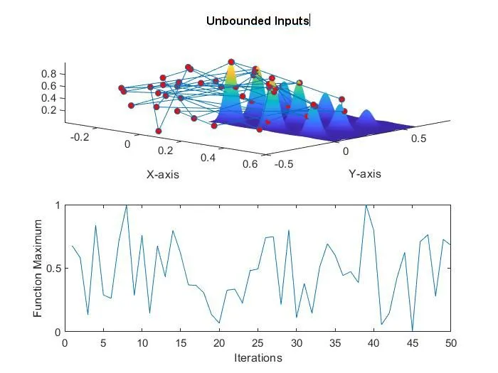
In the above plot, We can observe the random sampling of the Generic Algorithm generating a new optimum valvue for the function every time the code is run.
Study 2 : Bounded Condition with upper and lower limits defined
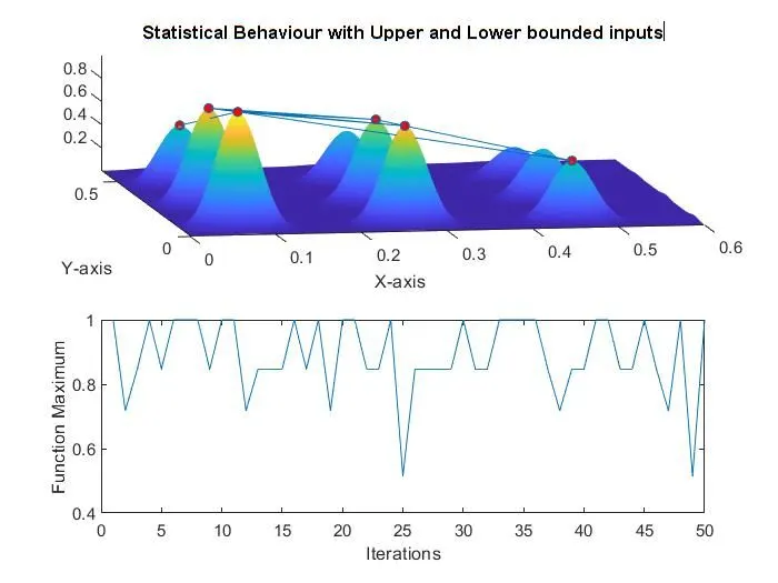
The above result shows the convergence of the x and y values. We can observe that the number of red dots are less compared to the earlier case study.
Study 3 : Condition of increasing the iterations in GA.
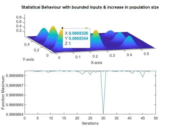
Here, we can observe only one point is visible when the number of iterations were increased to 350 and giving us the data of the maxima at (x,y,z) = (0.066,0.066,1) on the stalagmite.
References: