Week 3 - Solving second order ODEs
Aim: To Simulate the motion of a ODE representing the equation of motion of a simple pendulum with given constraints.
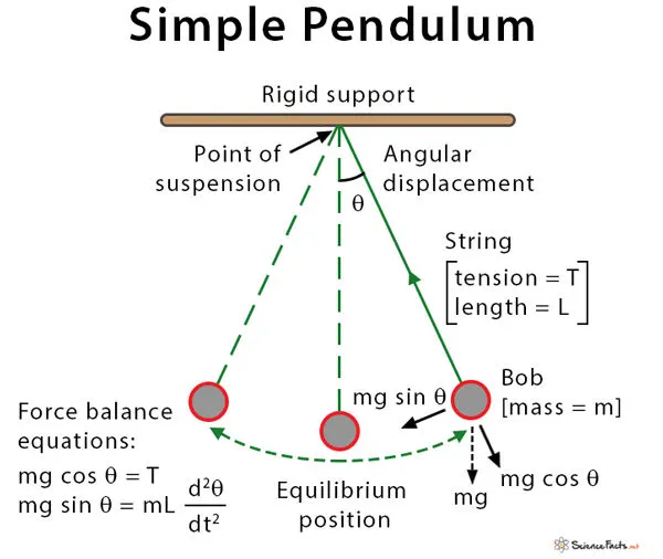
Theory: Simple pendulum can be described as a device where its point mass is attached to a light inextensible string and suspended from a fixed support. The vertical line passing through the fixed support is the mean position of a simple pendulum. The vertical distance between the point of suspension and the centre of mass of the suspended body (when it is in mean position) is called the length of the simple pendulum denoted by L. This form of the pendulum is based on the resonant system having a single resonant frequency.
A simple pendulum is a mechanical arrangement that demonstrates periodic motion. The simple pendulum comprises a small bob of mass ‘m’ suspended by a thin string secured to a platform at its upper end of length L.
The simple pendulum is a mechanical system that sways or moves in an oscillatory motion. This motion occurs in a vertical plane and is mainly driven by the gravitational force. Interestingly, the bob that is suspended at the end of a thread very light somewhat we can say it is even massless. The period of a simple pendulum can be made extended by increasing the length string while taking the measurements from the point of suspension to the middle of the bob. However, it should be noted that if the mass of the bob is changed it will the period remains unchanged. Period is influenced mainly by the position of the pendulum in relation to Earth as the strength of gravitational field is not uniform everywhere.
Meanwhile, pendulums are a common system whose usage is seen in various instances. Some are used in clocks to keep track of the time while some are just used for fun in case of a child’s swing. In some cases, it is used in an unconventional manner such as a sinker on a fishing line. In any case, we will explore and learn more about the simple pendulum on this page. We will discover the conditions under which it performs simple harmonic motion as well as derive an interesting expression for its period.
The Equation of the Simple Pendulum is given a follows
Figure 1: 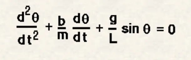
Now, We have to convert the second degree differential equation into a first order differential equation helping software to run the program. The conversion is done as follows.
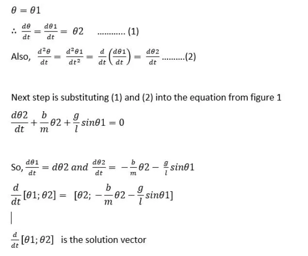
The above solution vector will be used in the function code which will be called in the main program. Function call is used to increase the readability, reusability of code leading to simplifying the major code helping in debugging if any bug occurs in the code during sloving.
The function code is written as follows:
%Function "ode_func" called to solve the ODE in main program

function [dtheta_dt] = ode_func(t,theta,b,g,l,m)

theta1 = theta(1);
theta2 = theta(2);
dtheta1_dt = theta2;
dtheta2_dt = -(b/m)*theta2 - (g/l)*sin(theta1);
dtheta_dt = [dtheta1_dt; dtheta2_dt]
end
Explination of ode45 function: ODE45 is usually a function of choice among the ODE solvers available in matlab. It compares methods of orders four and five to estimate error and determine step size. ODE45 is so accurate(medium accuracy) that it is used as a default to find the interpolations of the intermediate points of the ODE. Other usable ODE functions are: ODE23, ODE113 etc.
Main code of the silmulation:
%solving second order ODE of a pendulum

clear all
close all
clc

%Given Inputs
b = 0.05 %damping co-efficient
g = 9.81 %gravity acting on the body (m/s^2)
l = 1 % length of the spring(m)
m = 1 % mass of the body(kg)

%initial condition (Given)
%angular displacement is '0' and angular velocity is '3'

theta_0 = [0;3] %array representing the initial condition of the pendulum

%time span: Given to find the motion of the pendulum oscillating between 0-20 seconds
t_span = linspace(0,20,200) %Generates 200 values between 0 and 20

%solving ODE
[t,results] = ode45(@(t,theta) ode_func(t, theta, b, g, l, m), t_span, theta_0);

%plotting
figure(1)
hold on
plot(t, results(:,1))
plot(t,results(:,2))
title('Damped Harmonic motion of a Pendulum')
legend('Angular displacement','Angular velocity')
xlabel('Time(sec)')
ylabel('plot')

%for loop
ct = 1 %A counter value is defined to count frames
for i = 1:length(results(:,1))
    x_start = 0
    y_start = 0
    x_end = l*sin(results(i,1))
    y_end = l*cos(results(i,1))

    %plotting the animation
    figure(2)
    plot([-1 1], [0,0],'LineWidth',4)
    hold on
    plot([x_start x_end],[y_start y_end],'LineWidth',5)
    hold on

    plot(x_end,y_end,'Marker','o','MarkerSize',20,'MarkerFaceColor','y')
    title('Animation of transient behaviour of a Pendulum')
    axis([-1.5 1.5 -1.5 1.5])
    pause(0.001)
    hold off

    M(ct) = getframe(gcf) %Capturing the frames of the pendulum movement for given conditions
    ct = ct+1; %incrementing the counter
end

%Animation of the pendulum

movie(M) %Calling the frames
videofile = VideoWriter('Pendulum Animation invert.avi') %Writing the video
open(videofile) %Opening the file
writeVideo(videofile,M) %joining all frames to form video
close(videofile) %Close the video file
Error observed: 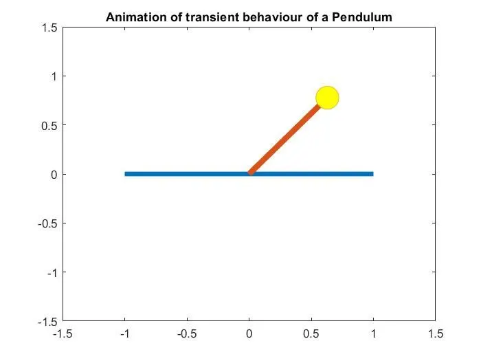
Rectification of code: Using “set(gca,'YDir','reverse')” we can invert the y axis grid values.
Final code: Eliminating the found error in the above code. The final code is written as follows:
%solving second order ODE of a pendulum

clear all
close all
clc

%Given Inputs
b = 0.05 %damping co-efficient
g = 9.81 %gravity acting on the body (m/s^2)
l = 1 % length of the spring(m)
m = 1 % mass of the body(kg)

%initial condition (Given)
%angular displacement is '0' and angular velocity is '3'

theta_0 = [0;3] %array representing the initial condition of the pendulum

%time span: Given to find the motion of the pendulum oscillating between 0-20 seconds
t_span = linspace(0,20,200) %Generates 200 values between 0 and 20

%solving ODE
[t,results] = ode45(@(t,theta) ode_func(t, theta, b, g, l, m), t_span, theta_0);

%plotting
figure(1)
hold on
plot(t, results(:,1))
plot(t,results(:,2))
title('Damped Harmonic motion of a Pendulum')
legend('Angular displacement','Angular velocity')
xlabel('Time(sec)')
ylabel('plot')

%for loop
ct = 1 %A counter value is defined to count frames
for i = 1:length(results(:,1))
    x_start = 0
    y_start = 0
    x_end = l*sin(results(i,1))
    y_end = l*cos(results(i,1))

    %plotting the animation
    figure(2)
    plot([-1 1], [0,0],'LineWidth',4)
    hold on
    plot([x_start x_end],[y_start y_end],'LineWidth',5)
    hold on

    plot(x_end,y_end,'Marker','o','MarkerSize',20,'MarkerFaceColor','y')
    set(gca,'YDir','reverse')
    title('Animation of transient behaviour of a Pendulum')
    axis([-1.5 1.5 -1.5 1.5])
    pause(0.001)
    hold off

    M(ct) = getframe(gcf) %Capturing the frames of the pendulum movement for given conditions
    ct = ct+1; %incrementing the counter
end

%Animation of the pendulum

movie(M) %Calling the frames
videofile = VideoWriter('Pendulum Animation.avi') %Writing the video
open(videofile) %Opening the file
writeVideo(videofile,M) %joining all frames to form video
close(videofile) %Close the video file
Result:
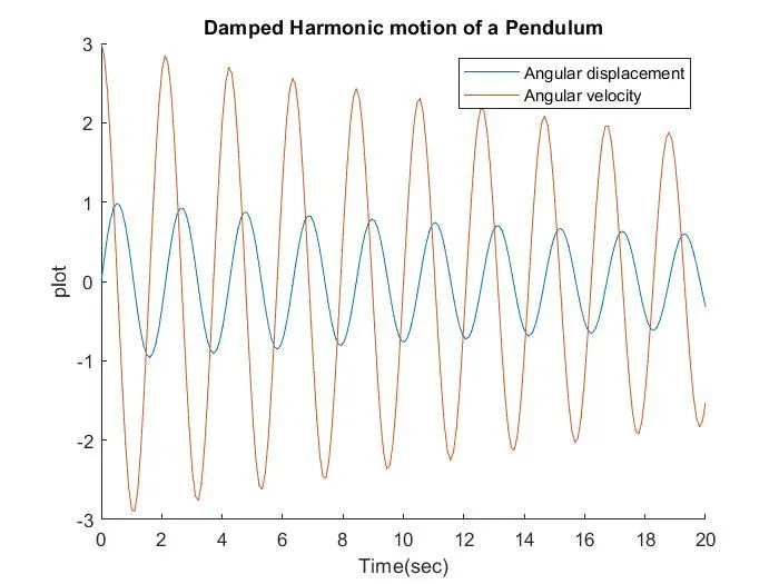
The graph shows the plot of angular displacement and angular velocity with respect to time decreasing gradually due to damping force acting on the body.
Animation: Refer link: https://drive.google.com/file/d/1Bm9O8-jJ1npny4JiLW5_9RObZ85jvHnP/view?usp=sharing