Week 4.1 - Genetic Algorithm

AIM : Find the global maxima using stalagmite function in Genetic Algorithm.

THEORY :

In computer science and operations research, a genetic algorithm (GA) is a metaheuristic inspired by the process of natural selection that belongs to the larger class of evolutionary algorithms (EA). Genetic algorithms are commonly used to generate high-quality solutions to optimization and search problems by relying on biologically inspired operators such as mutation, crossover and selection. Some examples of GA applications include optimizing decision trees for better performance, automatically solve Sudoku puzzles, hyper parameter optimization, etc.

Find minimum of function using genetic algorithm

collapse all in page

Syntax

x = ga(fun,nvars)

x = ga(fun,nvars,A,b)

x = ga(fun,nvars,A,b,Aeq,beq)

x = ga(fun,nvars,A,b,Aeq,beq,lb,ub)

x = ga(fun,nvars,A,b,Aeq,beq,lb,ub,nonlcon)

x = ga(fun,nvars,A,b,Aeq,beq,lb,ub,nonlcon,options)

x = ga(fun,nvars,A,b,Aeq,beq,lb,ub,nonlcon,intcon)

x = ga(fun,nvars,A,b,Aeq,beq,lb,ub,nonlcon,intcon,options)

fun = the objective function

nvars = the dimension of fun

A = subject to the linear inequalities constraints

b = subject to the linear inequalities constraints

Aeq = subject to the linear equalities constraints

beq = subject to the linear equalities constraints

ub = upper bound

lb = lower bound

nonlcon = nonlinear constraints

options = the default optimization parameters

intcon = integer values

Choosing a Fitness Function

To start off, there must be a fitness function that measures how well a set of input parameters perform. Solutions with a higher fitness derived from a fitness function will be better than ones with a lower fitness. This fitness function will generate a fitness value for each set of input parameters and is used to evaluate how well each set of parameters perform.

Generate a Population

To run a genetic algorithm, first start off with a population of individuals where each individual is a solution. The solution is represented with a set of genes where each gene in the solution is a variable within the model. Each solution is randomly generated and evaluated against the fitness function to generate a fitness score. It is very important to choose an appropriate population size. If the population size is too low, then it is much harder to explore the entire state space of the problem. If the population is too large, then it will take a very long time to process each generation as system costs for calculating fitness and generating each population will take exponentially more time to process.

Parent Selection

Next, the population goes through a process called parent selection where the best solutions (most fit individuals) will be selected to create the next generation of solutions. There are many ways to do this, such as Fitness-Proportion Selection (FPS), Rank-Based Selection, and Tournament Selection. These methods all have their pros and cons and should be picked based on the model.

Crossover

Once the parents have been selected, the parents undergo a process called crossover. Crossover is when two parents crossover their genes in order to create a new solution (also known as a child). This promotes exploration in the state space of the problem and potentially generates new solutions that have never been tested before.

Mutation

After the crossover phase, the children generated goes through a mutation phase. Mutation is when each gene could potentially change according to a random probability. This allows for exploitation as the children solution will not change as drastically as during the crossover phase but will still be able to explore around the neighbourhood of its current solution.

Survivor Selection

Once the children population is created, the next stage is survivor selection. This is the stage that decides which individuals get to move on to the next generation. There are multiple ways to do this as the new generation can be selected from both the pool of parents and the pool of children. There are two main methods to select the survivors of each generation, Age-Based Selection and Fitness-Based Selection (FBS). In FBS, there is Elitism, where the most fit of every population is selected, and Genitor, where the worst fit of every population gets eliminated.

Algorithm Repetition

Once the new generation is selected, this whole process repeats until the algorithm converges based off of some convergence criteria. After the whole algorithm runs, the best solution from all of the generations is returned.

Solution Procedure :

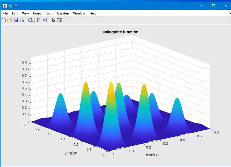
• X & Y values are assumed to be in ranges of 0 to 0.6 and the meshgrid is used to create 2D arrays for xx & yy.
• We utilize the stalagmite function to generate the 3rd dimension corresponding to the x & y value.
• In the stalagmite function, the order obtained to global maxima will multiply the output of the function by -1 .
• of iterations GA is assumed to be 50.

MATLAB Program :

clear all
close all
clc

% for dividing 0 to 0.6 in 150 parts

x = linspace(0,0.6,150);
y = linspace(0,0.6,150);

% Converting into 2D array

[xx yy] = meshgrid(x, y);

rep = 50;

% Calculating Study time

tic

for i = 1:length(xx)

    for j = 1:length(yy)

        input_vector(1) = xx(i,j);
        input_vector(2) = yy(i,j);
        f(i,j) = stalagmite(input_vector);

    end
end

study_time = toc

% Ploting 

surfc(xx,yy,-f)
% For Smooth 3D graph
shading interp
% Leveling
xlabel('x value')
ylabel('y value')
% Title Name
title ('stalagmite function')

%-----------------------------------------------------------------------------------
%STUDY 1

tic
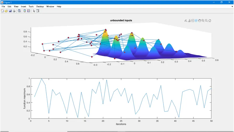
for i = 1:rep

    [inputs, fopt(i)] = ga(@stalagmite,2);
    xopt(i) = inputs(1);
    yopt(i) = inputs(2);

end
study_time1 = toc

figure(1)
subplot(2,1,1)
hold on
surfc(x,y,-f)
shading interp
plot3(xopt,yopt,-fopt,'marker','o','MarkerSize',6,'MarkerFaceColor','r')
title('unbounded inputs')
subplot(2,1,2)
plot(-fopt)
xlabel('iterations')
ylabel('function maximum')

% --------------------------------------------------------------------
% STUDY 2

tic

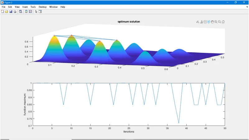
for i = 1:rep

    [inputs,fopt(i)] = ga(@stalagmite,2,[],[],[],[],[0;0],[0.6;0.6]);
    xopt(i) = inputs(1);
    yopt(i) = inputs(2);

end

study_time2 = toc

figure(2)
subplot(2,1,1)
hold on
surfc(x,y,-f)
shading interp
plot3(xopt,yopt,-fopt,'Marker','o','MarkerSize',5,'MarkerEdgeColor','r');
title('optimum solution')
subplot(2,1,2)
plot(-fopt)
xlabel('iterations')
ylabel('function maximum')

%-------------------------------------------
% STUDY 3

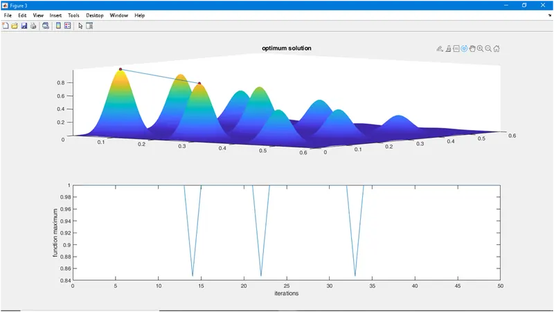
options = optimoptions(@ga)
options = optimoptions(options,'PopulationSize',170);

tic
for i = 1:rep

    [inputs,fopt(i)] = ga(@stalagmite,2,[],[],[],[],[0;0],[1;1],[],[],options);
    xopt(i) = inputs(1);
    yopt(i) = inputs(2);

end

study_time3 = toc

figure(3)
subplot(2,1,1)
hold on
surfc(x,y,-f)
shading interp
plot3(xopt,yopt,-fopt,'marker','o','MarkerSize',5,'MarkerFaceColor','r');
title('optimum solution')
subplot (2,1,2)
plot(-fopt)
xlabel('iterations')
ylabel('function maximum')

% Global Optimization
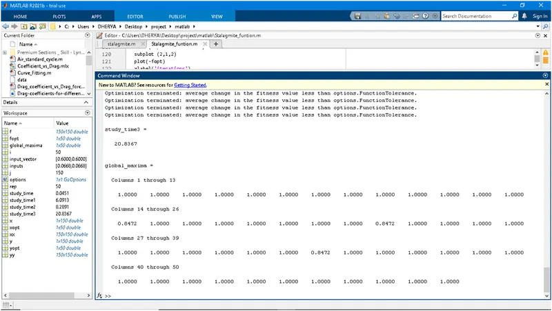
global_maxima = -fopt

Formula for Stalagmite Function :

`f(x,y)= f_(1,x) f_(2,x) f_(1,y) f_(2,y)`

where ,

`f_(1,x)=〖[sin⁡(5.1πx+0.5)]〗^6`

`f_(1,y)=〖[sin⁡(5.1πy+0.5)]〗^6`

`f_(2,x)=exp⁡[-4ln⁡(2) (x-0.0667)^2/0.64]`

`f_(2,y)=exp⁡[-4ln⁡(2) ((y-0.0667)^2)/0.64]`

Program for Stalagmite Function :

function [f] = stalagmite(input_vector)
x = input_vector(1);
y = input_vector(2);

f1 = (sin(5.1*pi*x + 0.5)).^6;
f2 = exp(-4*log(2)*((x- 0.0667).^2)./0.64);
f3 = (sin(5.1*pi*y + 0.5)).^6;
f4 = exp(-4*log(2)*((y- 0.0667).^2)./0.64);

f = -(f1*f2*f3*f4);

end

Results :