Week 3 - Solving second order ODEs
AIM : Solving second order Differenctial Equestion using MATLAB
OBJECTIVE :
- To write a program that solves the following ODE.
- To animate the motion of the pendulum.
THEORY :
An ordinary differential equation (also abbreviated as ODE), in Mathematics, is an equation which consists of one or more functions of one independent variable along with their derivatives. A differential equation is an equation that contains a function with one or more derivatives. But in the case ODE, the word ordinary is used for derivative of the functions for the single independent variable. In case of other types of differential equations, it is possible to have derivatives for functions more than one variable. The types of DEs are partial differential equation, linear and non-linear differential equations, homogeneous and non-homogeneous differential equation.
DEFINATION :
In mathematics, the term “Ordinary Differential Equations” also known as ODE is an equation that contains only one independent variable and one or more of its derivatives with respect to the variable. In other words, the ODE is represented as the relation having one independent variable x, the real dependent variable y, with some of its derivatives.
y’,y”, ….yn ,…with respect to x.
A pendulum is a weight suspended from a pivot so that it can swing freely. When a pendulum is displaced sideways from its resting, equilibrium position, it is subject to a restoring force due to gravity that will accelerate it back toward the equilibrium position. When released, the restoring force acting on the pendulum's mass causes it to oscillate about the equilibrium position, swinging back and forth. The time for one complete cycle, a left swing and a right swing, is called the period. The period depends on the length of the pendulum and also to a slight degree on the amplitude, the width of the pendulum's swing.
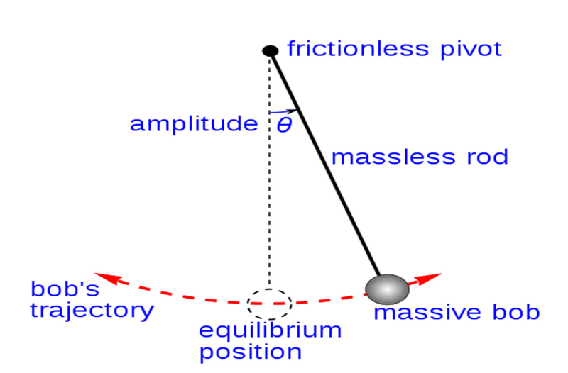
From the first scientific investigations of the pendulum around 1602 by Galileo Galilee , the regular motion of pendulums was used for timekeeping, and was the world's most accurate timekeeping technology until the 1930s. The pendulum clock invented by Christiaan Huygens in 1658 became the world's standard timekeeper, used in homes and offices for 270 years, and achieved accuracy of about one second per year before it was superseded as a time standard by the quartz clock in the 1930s. Pendulums are also used in scientific instruments such as accelerometers and seismometers. Historically they were used as gravimeters to measure the acceleration of gravity in geo-physical surveys, and even as a standard of length. The word "pendulum" is new Latin, from the Latin pendulus, meaning 'hanging'.
In general the motion of simple pendulum is considered to be simple harmonic with constant amplitude and is given by the equation,
`(d^2 θ)/(dt^2 )+θ/l sinθ=0`
Where,
`theta`= angular displacement ;
g = acceleration due to gravity in m/sec2;
`l`= length of the pendulum in m.
In real condition , every pendulum subjected restoring force to damp the motion and the differential equation for mtion of pendulum with damping is as follows,
`(d^2 θ)/〖dt〗^2 +b/m (dθ/dt)+θ/l sinθ=0`
Where,
`b`= damping coefficient;
`m`= mass of bob in kg.
Derivation for code simplification-
Let `θ=θ_1`
Then, `dθ/dt=〖dθ〗_1/dt=θ_2` and
`(d^2 θ)/〖dt〗^2 =(d^2 θ_1)/〖dt〗^2 =d/dt(〖dθ〗_1/dt)=〖dθ〗_2/dt`
we get,
`〖dθ〗_2/dt+b/m θ_2+θ/l sinθ_1=0`
This is a first order equation, hence
`∴ 〖dθ〗_1/dt=θ_2`
`∴ 〖dθ〗_2/dt=-b/m θ_2-θ/l 〖sinθ〗_1`
`d/dt [■(θ_1@θ_2 )]=[■(θ_2@-b/m θ_2-g/l sinθ_1 )]`
Where ,
`theta_1`= Angular Displacement
`theta_2`= Angular Velocity
MATLAB PROGRAM
% Simple Pendulum & Its Animation
clear all
close all
clc
% Given Inputs
b = 0.05; % damping coefficient
g = 9.81; % gravity in m/sec square
l = 1;    % Length of pendulum in m
m = 1;    % Mass of pendulum bob in Kg
theta_0 = [0;3]; % Angle range in radians
t_span = linspace(0,20,1000); % Time span from 0 to 20 sec
% Solving ODE
[t,solution] = ode45(@(t,theta) pendulum_ode(t,theta,b,g,l,m),t_span,theta_0 );
% Plotting Angular displacement and Angular Velocity against time
plot(t,solution(:,1),'LineWidth',3);
hold on
plot(t,solution(:,2),'LineWidth',3);
axis([0 20 -4 4])
ylabel('Amplitute')
xlabel('Time in (seconds)');
title('Damping in Simple Pendulum');
legend('Angular Displacement','Angular Velocity');
pause(18);
ct = 1;
for i = 1:length(t_span);

    x0 = 0;
    y0 = 0;

    x1 = l*sin(solution(i,1));
    y1 = -1*cos(solution(i,1));

    % Simulation of motion of Simple Pendulum

    plot([x0 x1],[y0 y1],[-0.5,0.5],[0 0],'LineWidth',3);

    hold on

    plot(x1,y1,'Marker','o','MarkerSize',25,'MarkerFaceColor','r')
    axis([-1.5 1.5 -1.5 0.5])
    grid on
    title('Motion of Simple Pendulum with Damping')
    pause(0.005)
    M(ct) = getframe(gcf) ;
    ct = ct + 1;
    hold off
end
% Animation of Motion of Pendulum

movie(M)
videofile = VideoWriter('Simple_pendulum_motion','Uncompressed AVI');
open(videofile)
writeVideo(videofile,M)
close(videofile)
** The function for second order ODE ,’ pendulum_ode’ is created by following codes,
function [dtheta_dt] = pendulum_ode(t,theta,b,g,l,m)
theta1 = theta(1);
theta2 = theta(2);
dtheta1_dt = theta2;
dtheta2_dt = -(b/m)*theta2 - (g/l)*sin(theta1);
dtheta_dt =[dtheta1_dt;dtheta2_dt];
end
*** This function is based on matrix form, ode45 is inbuilt function of Matlab to compare 4th & 5th order method to estimate error and determines step size.
****Program Output :
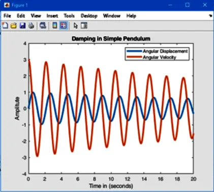
RESULT :
# The curve displacement and velocity reduces w.r.t time, only due to damping factor. That’s why its called damped dimple harmonic motion.
## From animation we conclude that;
`Damping coefficient∝ 1/(motion of pendulum)`
ERRORS :
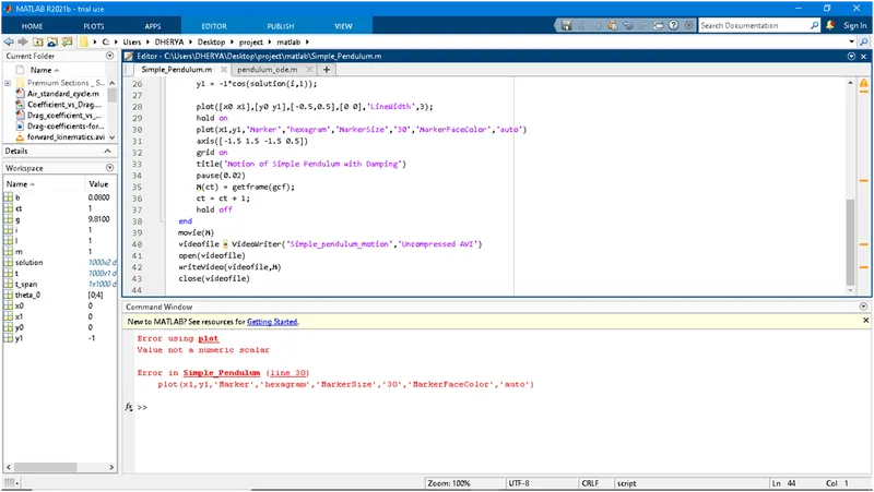
Solution = numeric values are not put in inverted commas
My movie link is https://drive.google.com/file/d/1metX3jVFEqOyfao31H_ElecrjxVhvNKa/view?usp=sharing